Estimating the gravitational acceleration constant using Raspberry Pi, IR proximity sensors, and the least-squares method – Fusion of Engineering, Control, Coding, Machine Learning, and Science

In this post, we present a simple experimental setup for estimating the gravitational acceleration constant. The gravitational acceleration is estimated using a least-squares method. The data acquisition and computations are performed using a Raspberry Pi (RP) microcontroller. A video about this post is given below.

The working principle of the experimental setup is shown in Fig.1 below.

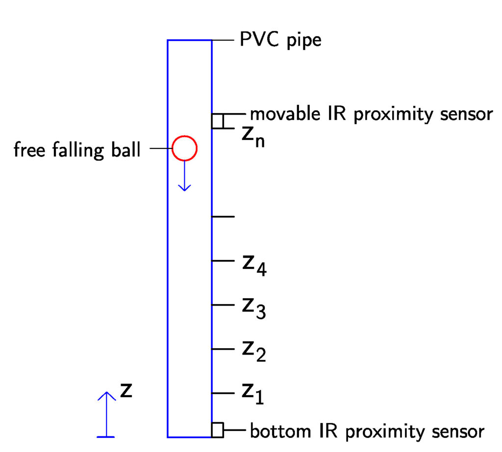
Figure 1: The working principle of the experimental setup for estimating the gravitational acceleration.

A (tennis) ball freely falls in a PVC pipe. The PVC pipe has ball openings and sensor mounts at prescribed heights $z_{i}$ , $i=1,2,3, \ldots, n$ . At the bottom of the pipe, an InfraRed (IR) proximity sensor is mounted. We use OSOYOO low-cost IR proximity sensors whose specs can be found here. The sensor output is a digital signal (HIGH or LOW voltage) depending on the proximity of the object. Another IR proximity sensor is placed at prescribed heights $z_{i}$ . Using an RP microcontroller we measure the time between the activations of the upper and lower sensors. This time, denoted by $t_{i}$ , is approximately equal to the time it takes for the ball to fall from the height $z_{i}$ .

The estimation problem can be formulated as follows. From the set of measurements ${(t_{i},z_{i}), i=1,2,\ldots, n}$ , estimate the gravitational acceleration constant.

Next, we derive the equation of motion of the free-falling ball. The second Newton’s law governs the motion of the ball:

(1) $\begin{align*}m\vec{a}=m\vec{g}\end{align*}$

(2) $\begin{align*}\vec{a}=\vec{g}\end{align*}$

where $\vec{a}$ is the second derivative of the position $z$ (acceleration) and $g$ is the gravitational acceleration constant. The equation \eqref{ equationOfMotion2 } is a vector equation. By scalarly multiplying this equation by the unit vector of the $z$ axis, we obtain the following equation:

(3) $\begin{align*}\ddot{z}=-g\end{align*}$

By integrating this equation two times, and by taking into account the initial condition $\dot{z}(0)=0$ and $z(0)=z_{i}$ , we obtain the following equation:

(4) $\begin{align*}z(t)=-g \frac{t^{2}}{2}+z_{i}\end{align*}$

where $t$ is time. For $t=t_{i}$ the ball reaches the ground. Substituting $z(t_{i})=0$ in \eqref{finalEquation}, we obtain:

(5) $\begin{align*}z_{i}=g\frac{t^{2}_{i}}{2}\end{align*}$

This equation can be used to form the least-squares problem for estimating the constant $g$ . From \eqref{finalEquation2}, we have:

(6) $\begin{align*}\underbrace{\begin{bmatrix}z_{1} \\ z_{2} \\ \vdots \\ z_{n} \end{bmatrix}}_{\mathbf{z}} = \underbrace{\begin{bmatrix} \frac{t^{2}_{1}}{2} \\ \frac{t^{2}_{2}}{2} \\ \vdots \\ \frac{t^{2}_{n}}{2} \end{bmatrix}}_{\mathbf{w}} g\end{align*}$

where $\mathbf{z} \in \mathbb{R}^{n}$ and $\mathbf{w} \in \mathbb{R}^{n}$ are the height and transformed time vectors. In practice, when $t_{i}$ are measurements, the last equation is not satisfied exactly. That is, the equation has the following form:

(7) $\begin{align*}\mathbf{z}=\mathbf{w}g+\mathbf{e}\end{align*}$

where $\mathbf{e}\in \mathbb{R}^{n}$ is the noise vector. The estimate of $g$ is found by solving the following optimization problem:

(8) $\begin{align*}\min_{g} \left\| \mathbf{z}-\mathbf{w}g \right\|_{2}^{2}\end{align*}$

where $\left\| \cdot \left\|_{2}$ denotes the 2-norm.

The solution is given by:

(9) $\begin{align*}\hat{g}=\big( \mathbf{w} ^{T} \mathbf{w} \big)^{-1} \mathbf{w} ^{T} \mathbf{z}\end{align*}$

where $\big(\cdot \big)^{-1}$ denotes the matrix inverse operation and $\big(\cdot \big)^{T}$ is the matrix transpose.

Rendered by QuickLaTeX.com

The MATLAB code for calculating the g constant is given below.

g_true=9.80665;
data=[0.2   1     0.1539    0.171467;
     0.4   2   0.250098  0.244594;
     0.6   3   0.324306  0.320726;
     0.8   4   0.383247  0.40603 ;
     1     5    0.443352  0.437858;
     1.2     6    0.493963  0.508561;
     1.4     7    0.542227  0.542927;
     1.6     8    0.577312  0.570544;
     1.8     9    0.598127  0.603123;
     2       10   0.664753   0.650943;];
 

 w_est=data(:,3).^2/2;
 w_val=data(:,4).^2/2;
 z =data(:,1)+0.01;
 
 g=inv(w_est'*w_est)*(w_est'*z)
 
 error=((g_true-g)/g_true)*100

The estimation error is 0.5 %. Notice that on line 16 we added an additional centimeter to the height vector. This is has been done to take into account the fact that the sensors are placed 1cm below the point from which the ball falls (for more details see the video). The C/C++ code for obtaining the measurements is given below.

/*
 / Andrew Brennan
 / Nicholas Doherty
 / Prof. Aleksandar Haber, PhD
 / Verifying Earth's Gravitational Acceleration
 / CUNY College of Staten Island
 / 6/19/2019
 / 
*/
#include <wiringPi.h>
#include <iostream>
#include <ctime>
 
using namespace std;

int main(void)
{
	
	clock_t startTime;
	clock_t endTime;
	double duration = 0;
	
	int sensor_upper_pin = 0; // Set upper sensor pin.
	int sensor_lower_pin = 2;// Set lower sensor pin.
		
	int sensor_upper = 0;
	int sensor_lower = 0;
	
	int iteration_num = 0;
	
	wiringPiSetup();

	pinMode(sensor_upper_pin, INPUT); // Set upper sensor to input.
	pinMode(sensor_lower_pin, INPUT); // Set lower sensor to input.

	while(1)
		{
		sensor_upper = digitalRead(sensor_upper_pin); // Continually check upper sensor for input.
		if (sensor_upper == 0) // When ball passes upper sensor,
			{
			startTime = clock(); // start clock.
			sensor_lower = digitalRead(sensor_lower_pin); // Continually check lower sensor for input.
			
			while (sensor_lower == 1) // While no input from lower sensor.
				{
				sensor_lower = digitalRead(sensor_lower_pin); // Do nothing.
				}
			
			endTime = clock(); // Stop clock when ball passes lower sensor.
			duration = (endTime - startTime) / (double) CLOCKS_PER_SEC; // Calculate time difference between readings.
			
			iteration_num++;
			cout<<"\nIteration "<<iteration_num<<".\nTime between sensor detections: "<<duration<<" seconds."<<endl; // Output duration.
			}
		}
return 0;
}

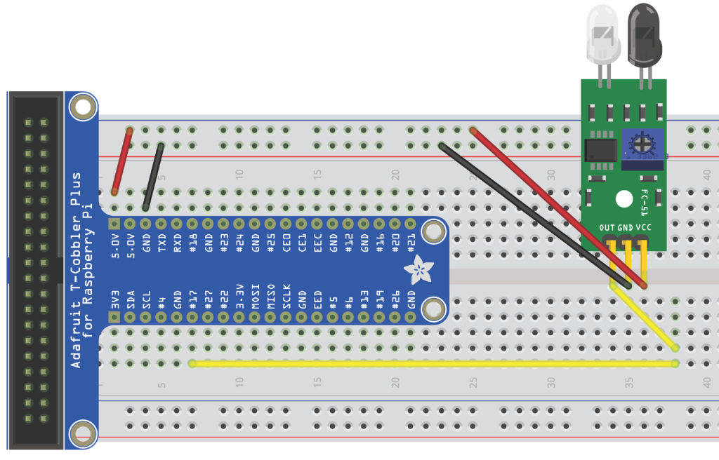
The wiring diagram for one sensor is shown below. Notice that that the power pin of the sensor should be attached to the external power supply.

admin

You might also like

Some questions for the midterm exam

Controlling Servomotors using Raspberry Pi – 2

Plotting in Python – Single Plots and Subplots – Almost Everything You Need to Know