Mobile Robot Localization Using Extended Kalman Filter – Part I: Problem Formulation – Fusion of Engineering, Control, Coding, Machine Learning, and Science

In this control theory, mobile robotics, and estimation tutorial we explain how to develop and implement an extended Kalman filter algorithm for localization of mobile robots. We explain how to use the extended Kalman filter to localize (estimate) the robot location and orientation (location and orientation are called the robot pose). We also explain how to implement the localization algorithm in Python from scratch. Here, we need to immediately state that the localization algorithm is developed under the assumption that the locations of external landmarks (markers) are known and that the landmark measurement correspondence is also known. In our second tutorial series, we will consider the case when the landmark measurement correspondence is not known, and in the third tutorial series, we will consider the case when both the landmark locations and their measurement correspondence are not known. Do not be confused if you currently do not understand what is landmark or what is landmark measurement correspondence. These terms will be explained in this tutorial series.

Due to the objective complexity of the estimation and localization problems, we split this tutorial series into three parts:

Part I – You are currently reading the first part. In this part, we clearly explain the problem formulation. We explain what is a localization problem. We then explain what are landmarks (markers), and we explain the difference between localization with known landmarks and unknown landmarks. We summarize the mobile robot model, as well as its odometry model. We introduce the measurement model that provides us with information about the robot’s location with respect to the known landmarks.
Part II – In part two, whose link is given here, on the basis of the problem formulation given in the first part, we explain how to mathematically solve the robot localization problem by using the extended Kalman filter. We thoroughly explain how to compute all the partial derivatives necessary to implement the extended Kalman filter.
Part III – In part three of this tutorial series, whose link is given here, we explain how to implement the extended Kalman filter for mobile robot localization in Python from scratch.

This first tutorial part is organized as follows. First, we briefly summarize the kinematics model of the robot used in this tutorial series, as well as its odometry model. Based on these two models we derive the state equation of the mobile robot. We then derive the output equation that takes into account relative measurements with respect to external landmarks. We then briefly explain the landmark correspondence problem. Finally, we present the robot localization problem formulation.

The YouTube tutorial accompanying the first part is given below.

Kinematics and Odometry Models of Mobile Robot-State Equation Derivation

In this tutorial series, in order not to blur the main ideas of robotic localization with too complex mobile robot models, we use a differential drive robot as our mobile robot. This is done since a differential drive robot has a relatively simple configuration (actuation mechanism) which results in a simple kinematics model. The main purpose of this tutorial is to explain the main principles and ideas of robot localization, without blurring the main ideas with complex robotic configurations or complex mathematical models. Of course, everything explained in this tutorial series can be generalized to more complex mobile robot configurations, and even to UAVs or autonomous driving vehicles. We thoroughly explained the model of the differential drive robot in our previous tutorials given here and here. In the sequel, we briefly summarize the model, and by using this model as well as the odometry model we derive the state equation for localization.

The differential drive (differential wheeled robot) is shown in the figure below.

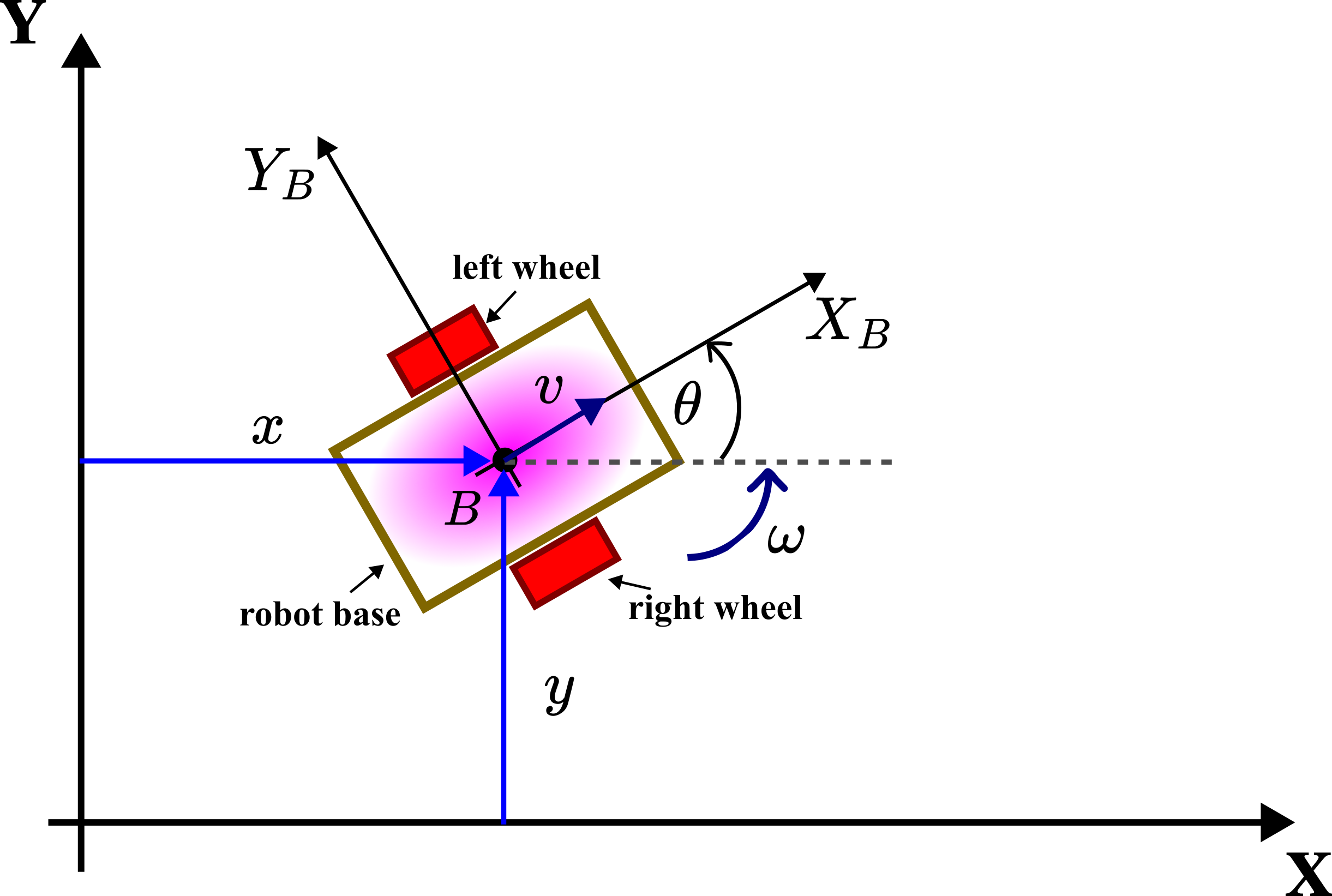
Figure 1: Top view of a differential drive (differential wheeled) mobile robot.

The robot consists of the robot base and two active (actuated) wheels. There is a third passive caster wheel that is not shown in this graph for clarity. The third caster wheel is used to provide support and stability for the robot base. The symbols used in the above figure are:

$X-Y$ is the fixed inertial coordinate system. This coordinate system is also called the inertial frame.
$X_{B}-Y_{B}$ is the body coordinate system. This coordinate system is also called the body frame. The origin of this coordinate system is at the point $B$ which is located at the center of the mass or the center of the symmetry of the mobile robot. The body frame is rigidly attached to the robot body, and it moves (translates and rotates) with the robot body.
$x$ and $y$ are the $X$ and $Y$ coordinates of the origin of the body frame. That is, these are the coordinates of the center of the body frame in the inertial coordinate system.
The angle $\theta$ is the angle that the $X$ axis of the inertial frame makes with the $X_{B}$ axis of the body frame. This angle is called the orientation angle.
The symbol $v$ denotes the instantaneous velocity of the body frame origin $B$ .
The symbol $\omega$ denotes the instantaneous angular velocity of the mobile robot.

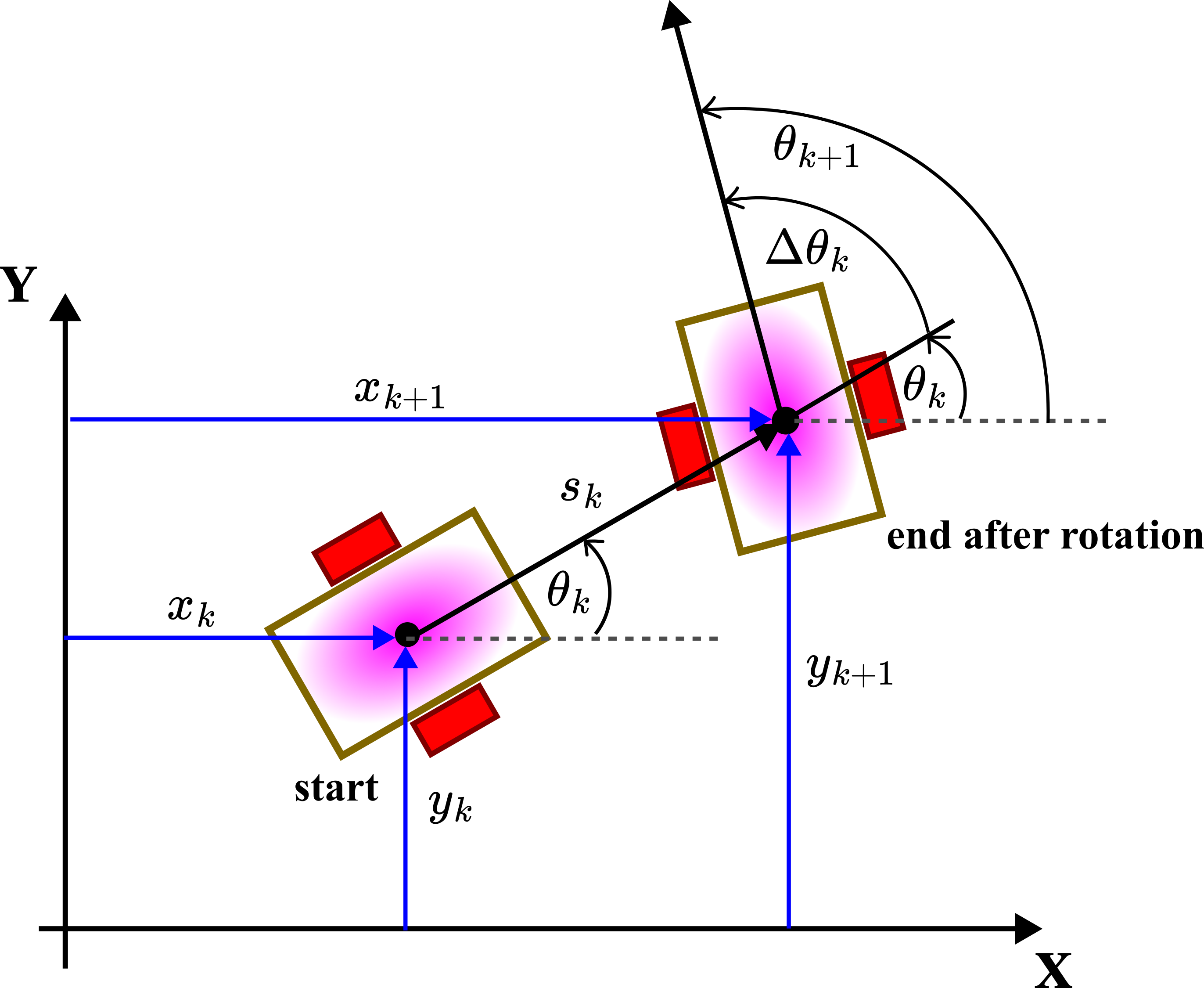
As explained in our previous tutorial given here, by discretizing the continuous-time kinematics of the mobile robot, we obtain the discrete-time model

(1) $\begin{align*}x_{k+1}& =x_{k}+s_{k}\cos(\theta_{k}) \\y_{k+1}& =y_{k}+s_{k}\sin(\theta_{k}) \\\theta_{k+1}& =\theta_{k}+\Delta \theta_{k}\end{align*}$

where (also see the figure shown below)

the subscript $k$ is the discrete-time instant.
$x_{k}$ and $y_{k}$ are the $x$ and $y$ coordinates at the discrete-time instant $k$ . That is, $x_{k}=x(kh)$ and $y_{k}=y(kh)$ , where $h$ is the discretization constant ( $h$ is the time interval between $k$ and $k+1$ ).
$s_{k}$ is the distance traveled by the robot between the time instants $k$ and $k+1$ in the direction of the velocity $v_{k}$ . It is assumed that the velocity is constant between the time instant $k$ and $k+1$ .
$\theta_{k}$ is the orientation at the discrete-time instant $k$ .
$\Delta \theta_{k}$ is the change of the orientation between the time instant $k$ and $k+1$ .

Figure 2: Motion of the robot between the discrete-time instants $k$ and $k+1$ .

Here, for simplicity, we assume that by using the odometry system, the following quantities are directly measured

The distance $s_{k}$ is measured.
The change of the angle $\Delta \theta_{k}$ is measured.

Instead of this assumption, we can assume that the velocity $v_{k}=s_{k}/h$ and angular velocity $\omega_{k}=\Delta \theta_{k}/h$ are measured directly.

Here, we need to explain the odometry process. We can measure the distance traveled $s_{k}$ by using wheel encoders or some other method. We can measure the angle change $\Delta \theta_{k}$ by using a gyroscope or a compass. However, due to the measurement imperfections and due to other mechanical phenomena, such as for example wheel slipping, we are not able to accurately measure both $s_{k}$ and $\Delta \theta_{k}$ . Instead, we measure

(2) $\begin{align*}\tilde{s}_{k}&=s_{k}+n_{s,k} \\\Delta \tilde{\theta}_{k}&=\Delta \theta_{k}+n_{\theta,k}\end{align*}$

where $n_{s,k}$ and $n_{\theta,k}$ are the measurement errors (measurement noise). We assume that both $n_{s,k}$ and $n_{\theta,k}$ are normally distributed with the standard deviations of $\sigma_{s}$ and $\sigma_{\theta}$ , respectively. From (2), we obtain

(3) $\begin{align*}s_{k}&=\tilde{s}_{k}-n_{s,k} \\\Delta \theta_{k}&=\Delta \tilde{\theta}_{k}-n_{\theta,k}\end{align*}$

By substituting (3) in (1), we obtain

(4) $\begin{align*}x_{k+1}& =x_{k}+(\tilde{s}_{k}-n_{s,k} )\cos(\theta_{k}) \\y_{k+1}& =y_{k}+(\tilde{s}_{k}-n_{s,k} )\sin(\theta_{k}) \\\theta_{k+1}& =\theta_{k}+\Delta \tilde{\theta}_{k}-n_{\theta,k}\end{align*}$

Let us separate noise from the states and measurements in the last set of equations

(5) $\begin{align*}x_{k+1}& =x_{k}+\tilde{s}_{k}\cos(\theta_{k})-n_{s,k} \cos(\theta_{k}) \\y_{k+1}& =y_{k}+\tilde{s}_{k}\sin(\theta_{k})-n_{s,k} \sin(\theta_{k}) \\\theta_{k+1}& =\theta_{k}+\Delta \tilde{\theta}_{k}-n_{\theta,k}\end{align*}$

Next, we formally define the states and inputs. The states are defined as follows

(6) $\begin{align*}z_{1,k}& = x_{k}\\z_{2,k}& = y_{k} \\z_{3,k}& = \theta_{k}\end{align*}$

The state vector is defined as follows

(7) $\begin{align*}\mathbf{z}_{k}=\begin{bmatrix} z_{1,k} \\ z_{2,k} \\ z_{3,k} \end{bmatrix}\end{align*}$

We define the inputs as follows

(8) $\begin{align*}u_{1,k}&=\tilde{s}_{k} \\u_{2,k}&=\Delta \tilde{\theta}_{k}\end{align*}$

Here, you should stop for a second, and try to understand the following. In (8), we defined actual measurements as inputs! However, readers with a strong background in control theory will find this assignment confusing. Usually, inputs in state-space models are control variables determined by an algorithm or determined by us. However, here, we define inputs as output measurements. That is, inputs are defined as measurements of the traveled distance and change of angle. This is a formal assignment that is often used in robotics literature. Also, these inputs are actually only observed at the time instant $k+1$ . This should always be kept in mind.

By substituting (6) and (8) in (5), we obtain

(9) $\begin{align*}z_{1,k+1}& =z_{1,k}+u_{1,k} \cos(z_{3,k})-n_{s,k} \cos(z_{3,k}) \\z_{2,k+1}& =z_{2,k}+u_{1,k} \sin(z_{3,k})-n_{s,k} \sin(z_{3,k}) \\z_{3,k+1}& =z_{3,k}+u_{2,k}-n_{\theta,k}\end{align*}$

Next, for clarity, we shift the time index from $k+1$ to $k$ in (9). As a result, we obtain the final form of the state equation

(10) $\begin{align*}z_{1,k}& =z_{1,k-1}+u_{1,k-1} \cos(z_{3,k-1})-n_{s,k-1}\cos(z_{3,k-1}) \\z_{2,k}& =z_{2,k-1}+u_{1,k-1} \sin(z_{3,k-1})-n_{s,k-1}\sin(z_{3,k-1}) \\z_{3,k}& =z_{3,k-1}+u_{2,k-1}-n_{\theta,k-1}\end{align*}$

This is the state equation that will be used for the development of the extended Kalman filter in the next tutorial. Here, it is very important to keep in mind the following when dealing with the state-space model (10). The measurement noise of the measured distance and change of angle formally act as process disturbance in (10). That is, when developing a state estimator, it should always be kept in mind that the stochastic part of the state equation involving $n_{s,k-1}$ and $n_{\theta,k-1}$ is not known. However, we know the distribution and standard deviations of these random variables. That is, we know the statistics of $n_{s,k}$ and $n_{\theta,k}$ . This statistics can be estimated from the collected data.

Next, we need to define the concept of landmarks (markers) and the output equation.

Landmarks (markers) and Output Equation

Localization will be formally defined in the next section of this tutorial. However, here we can briefly say that the localization is the process of estimating the robot pose vector $\mathbf{z}_{k}$ in (6) by using the available measurement data and the pose estimate from the previous time step. It is a very well-known fact that by only using the measurement of the traveled distance and the angle change (or by measuring the velocity and angular velocity) we cannot accurately localize the robot in space. That is, we cannot accurately estimate the robot pose by propagating in time the deterministic part of the state-space model (9). As the time interval of operation grows, the estimation error will also grow (estimation error variances will grow).

For that reason and to be able to accurately estimate the robot’s location and orientation in space, we need to introduce an additional sensor that is capable of measuring the distance and angle between the robot and external objects known as landmarks or markers in the robotics literature. We can define a landmark (marker) as an object or a feature of the environment that is used as a reference for measuring the robot’s location. Namely, we assume that a mobile robot is equipped with a sensor that can measure the distance between the robot and the landmark and the angle of the line connecting the robot and the landmark. This is illustrated in the figure below.

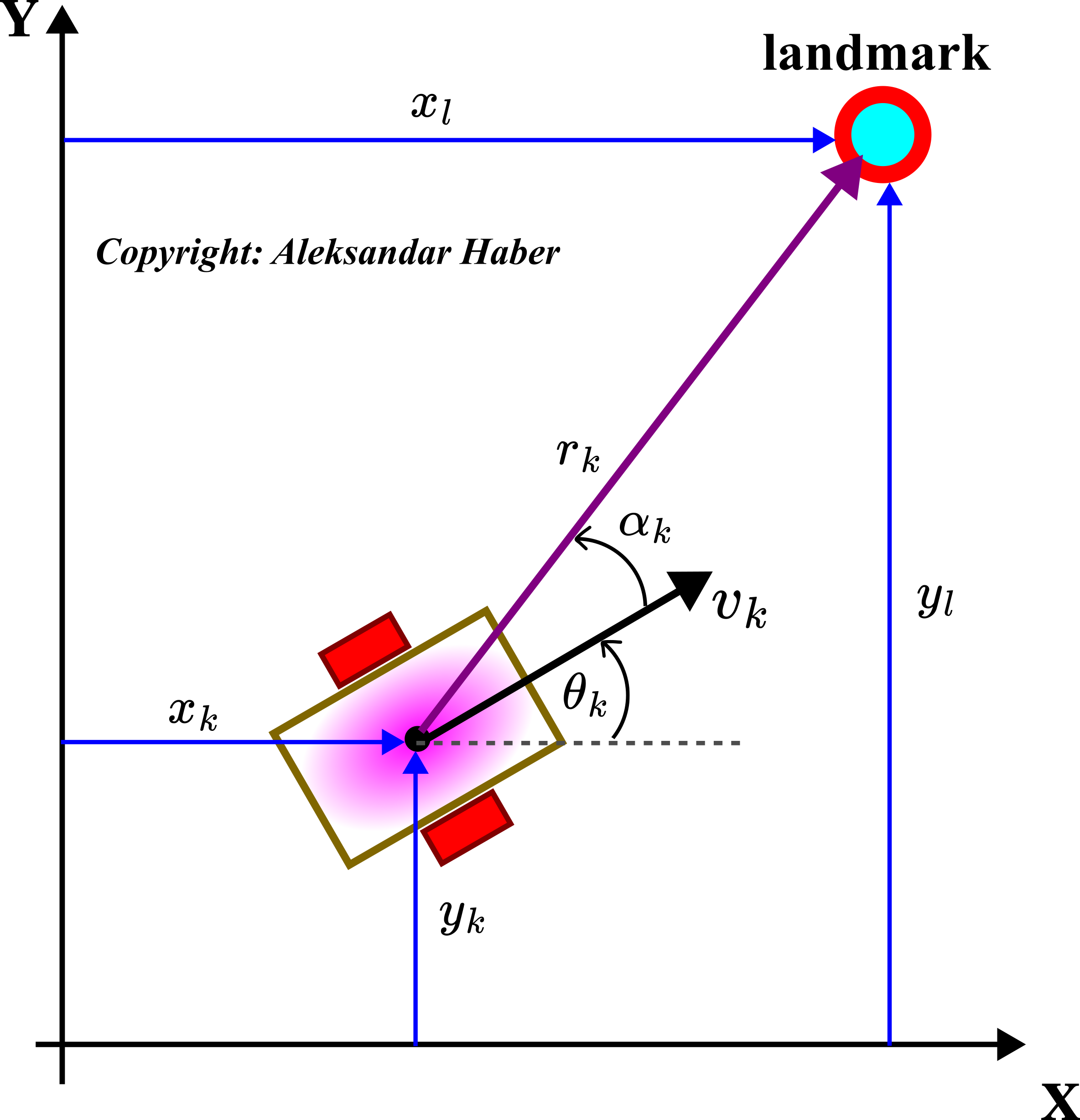
Figure 2: Landmark and measured distance and angle.

Figure above shows a landmark with the location $(x_{l},y_{l})$ , where $x_{l}$ and $y_{l}$ are the coordinates in the inertial coordinate system. The robot is equipped with a sensor that can measure

The distance $r_{k}$ at the discrete time instant $k$ between the origin of the body frame $B$ and the landmark. This distance is called the range.
Angle $\alpha_{k}$ at the discrete time instant $k$ . This angle is the angle between the line in the direction of the range (the line connecting the robot and landmark) and the heading direction of the robot marked by the velocity $v_{k}$ . The angle $\alpha_{k}$ is also called the bearing angle or simply bearing.

Here we make the following important assumption:

The location $(x_{l},y_{l})$ of every landmark in the inertial coordinate system is known accurately.

This assumption will be relaxed in our future tutorials on SLAM. Next, we need to define the measurement equation. From Fig. 2, it follows that the range $r_{k}$ can be expressed as follows

(11) $\begin{align*}r_{k}^{2} & =(x_{l}-x_{k})^{2}+(y_{l}-y_{k})^{2} \\r_{k} & =\sqrt{(x_{l}-x_{k})^{2}+(y_{l}-y_{k})^{2}}\end{align*}$

On the other hand, from the basic geometry we have

(12) $\begin{align*}\tan (\theta_{k}+\alpha_{k})& =\frac{y_{l}-y_{k}}{x_{l}-x_{k}} \\\theta_{k}+\alpha_{k} & =\text{atan2} \Big( \frac{y_{l}-y_{k}}{x_{l}-x_{k}} \Big) \end{align*}$

From the last equation, we have

(13) $\begin{align*}\alpha_{k} & =\text{atan2} \Big( \frac{y_{l}-y_{k}}{x_{l}-x_{k}} \Big) -\theta_{k}\end{align*}$

is the 2-argument arctangent function (here, it is important to use $\text{atan2}$ instead of the ordinary arctangent function). Next, we assume that the measurements of the range $r_{k}$ and the angle $\alpha_{k}$ are corrupted by the measurement noise, that is,

(14) $\begin{align*}r_{k} & =\sqrt{(x_{l}-x_{k})^{2}+(y_{l}-y_{k})^{2}}+n_{r,k} \\\alpha_{k} & =\text{atan2} \Big( \frac{y_{l}-y_{k}}{x_{l}-x_{k}} \Big) -\theta_{k}+n_{\alpha,k}\end{align*}$

where $n_{r,k}$ and $n_{\alpha,k}$ represent the measurement noise. We assume that both $n_{r,k}$ and $n_{\alpha,k}$ and normally distributed with the standard deviations of $\sigma_{r}$ and $\sigma_{\alpha}$ , respectively. By substituting the state assignment (6) in (14), we obtain

(15) $\begin{align*}r_{k} & =\sqrt{(x_{l}-z_{1,k})^{2}+(y_{l}-z_{2,k})^{2}}+n_{r,k} \\\alpha_{k} & =\text{atan2} \Big( \frac{y_{l}-z_{2,k}}{x_{l}-x_{1,k}} \Big) -z_{3,k}+n_{\alpha,k}\end{align*}$

The equations (15) represent the measurement model for a single landmark. However, we need to clarify what happens and how the measurement model is defined when we have more than a single landmark. That is, we need to define the landmark correspodence problem.

What is Landmark Correspondence Problem and Why It is Important

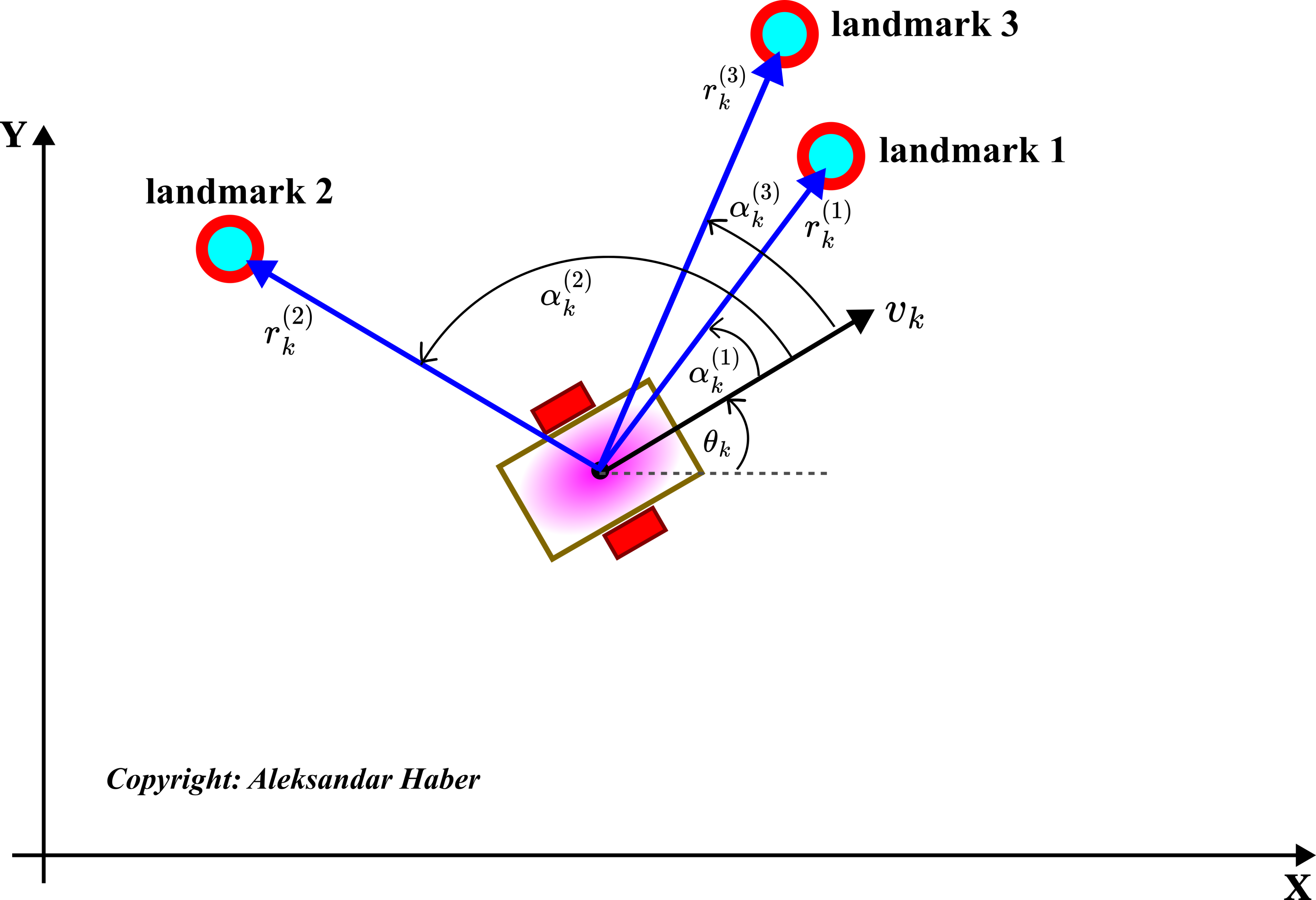
Consider the scenario shown in the figure below.

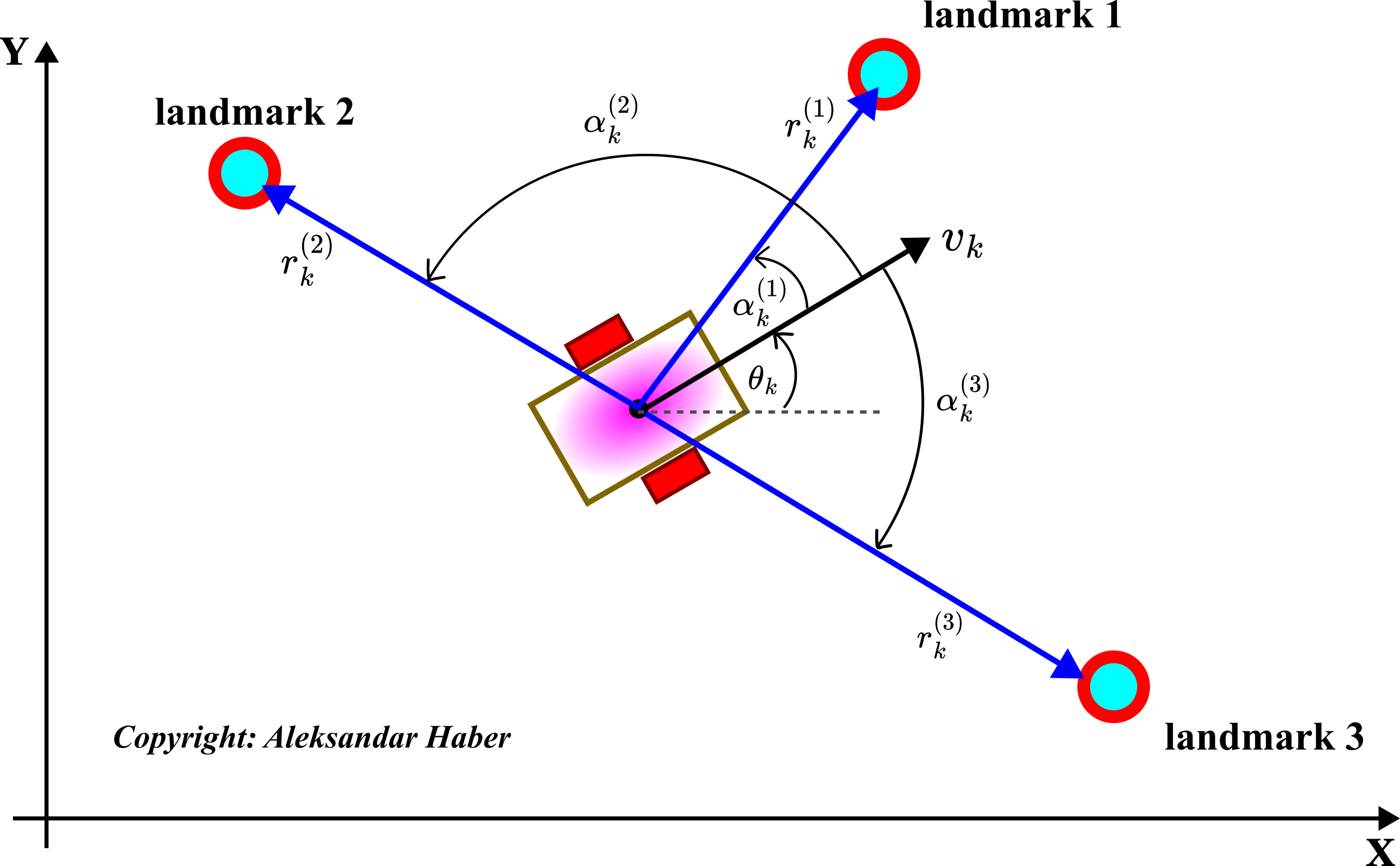
Figure 3: Mobile robot with three landmarks (markers).

The robot is in an environment with three landmarks. Let us suppose that we know the locations (coordinates) of all three landmarks. Furthermore, let us assume that the robot sensor can detect the range and bearings (angles) of three landmarks. What the robot receives are three measurements, where every measurement consists of a 2-tuple (range, bearing angle):

(16) $\begin{align*}& (r=0.3,\alpha=\frac{\pi}{6} ) \\& (r=0.55,\alpha=\frac{2\pi}{3}) \\& (r=0.6,\alpha=-\frac{\pi}{3})\end{align*}$

However, these measurements are unlabeled. Unlabeled means that the measurements are not assigned to the corresponding landmarks. That is, in the case of unlabeled measurements, we do not know the correspondence between the landmarks and measurements, and we cannot form the output equations (15). We need to assign every measurement tuple to the corresponding landmark, and after that, we need to form a single measurement equation (15) for every landmark.

The landmark correspondence problem is to assign the landmarks to the received measurements, that is, to label the received measurement tuples, where the label denotes the landmark that corresponds to the measurement. For example, in the case of Figure 3 above and the set of measurements (16), it is obvious that we have the following labels

(17) $\begin{align*}& (r=0.3,\alpha=\frac{\pi}{6} ) \rightarrow \text{landmark 1} \rightarrow \;\; r_{k}^{(1)}=0.3,\;\; \alpha_{k}^{(1)}=\frac{\pi}{6} \\& (r=0.55,\alpha=\frac{2\pi}{3}) \rightarrow \text{landmark 2} \rightarrow \;\; r_{k}^{(2)}=0.55 \;\; \alpha_{k}^{(2)}=\frac{2\pi}{3} \\& (r=0.6,\alpha=-\frac{\pi}{3}) \rightarrow \text{landmark 3} \rightarrow \;\; r_{k}^{(3)}=0.6,\;\; \alpha_{k}^{(2)}=-\frac{\pi}{3}\end{align*}$

The landmark labeling and correspondence in the figure are obvious since the landmarks are decently separated. Consequently, on the basis of the current robot location and received measurements, we can easily figure out how to label the measurements. However, in contrast, consider the landmark configuration shown below.

Figure 4: Mobile robot with three landmarks (markers) where two landmarks are close to each other.

In Fig. 4 above, landmark 3 and landmark 1 are close to each other. Consequently, the measurements might look like this

(18) $\begin{align*}& (r=0.3,\alpha=\frac{\pi}{6} ) \\& (r=0.55,\alpha=\frac{2\pi}{3}) \\& (r=0.6,\alpha=\frac{\pi}{5})\end{align*}$

Taking into account that the pose of the robot has to be estimated together with determining the landmark correspondence, and taking into account that all the measurements (including the robot odometry measurements) are corrupted by the measurement noise, it is difficult to properly assign the landmark labels to first and third measurements. That is, we are not sure how to assign landmark 1 and landmark 3 to these measurements.

The correct solution of the landmark correspondence problem is far from trivial and it will be addressed in our future tutorials. In this tutorial series, we assume that the received measurements are properly labeled. That is, in this tutorial series, we assume that the landmark correspondences are perfectly known.

Localization Problem for Mobile Robotics With Known Landmark Correspondence (Labels)

Now, we are ready to formulate the localization problem for mobile robots.

Let us assume that

There are $N$ fixed landmarks in the environment surrounding the mobile robot.
The locations of $N$ landmarks are known in the inertial coordinate frame. That is, the location $(x_{l,i},y_{l,i})$ of every landmark $i$ , where $i=1,2,3,\ldots, N$ , is known.
The mobile robot is equipped with a sensor that can measure the range $r^{(i)}_{k}$ and the bearing angle $\alpha_{k}^{(i)}$ of every landmark.
The landmark correspondences are perfectly known.
The robot is equipped with odometry sensors that can measure the traveled distance $\tilde{s}_{k}$ and robot orientation change $\Delta \tilde{\theta}_{k}$ .

Then, by using information about

The odometry readings $\tilde{s}_{k-1}$ and $\Delta \tilde{\theta}_{k-1}$ obtained at the discrete-time instant $k$ .
Landmark measurements $(r^{(1)}_{k},\alpha^{(1)}_{k})$ , $(r^{(2)}_{k},\alpha^{(2)}_{k})$ , $(r^{(3)}_{k},\alpha^{(3)}_{k})$ , $\ldots$ , $(r^{(N)}_{k},\alpha^{(N)}_{k})$ obtained at the discrete-time instant $k$ .
The pose estimate computed at the previous discrete-time step $k-1$ : $\hat{x}_{k-1}, \hat{y}_{k-1}$ and $\hat{\theta}_{k-1}$

at the discrete-time instant $k$ estimate the pose of the robot: $\hat{x}_{k}, \hat{y}_{k}$ and $\hat{\theta}_{k}$ .

This problem formulation is graphically illustrated in the figure below.

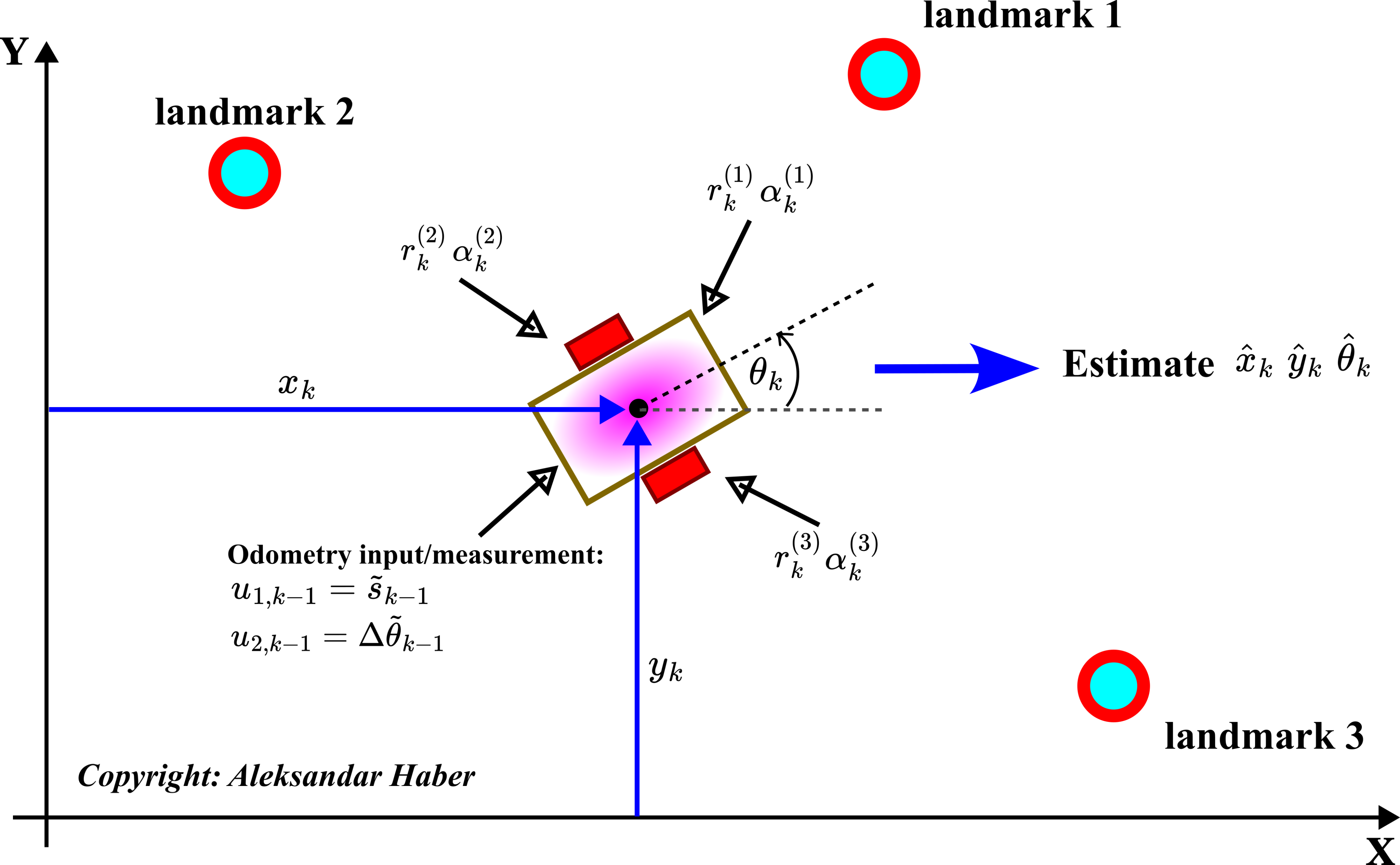
Here are several important comments about this problem formulation.

First of all, estimates of the quantities are denoted with the hat notation: $\hat{x}_{k}, \hat{y}_{k}$ and $\hat{\theta}_{k}$ . Then, the third assumption can be made more realistic by assuming that we can only obtain the landmark measurements if the distance between the robot and the landmark is such that the landmark is in the sensor range. For example, some low-cost lidars have a measurement range of about 10-15 meters, and we can obtain the landmark information only if the landmark is in this range. In the next tutorial part, we will investigate the performance of the extended Kalman filter when all the landmarks can be observed at every time instant $k$ and when only landmarks in a given sensor range can be observed at the given discrete-time instant.

Kinematics and Odometry Models of Mobile Robot-State Equation Derivation

Landmarks (markers) and Output Equation

What is Landmark Correspondence Problem and Why It is Important

Localization Problem for Mobile Robotics With Known Landmark Correspondence (Labels)

admin

You might also like

What is Dead Reckoning – Clear Explanation with Python Simulation – Part I

Automatic State-Space Derivation and Simulation of Nonlinear Dynamical Systems in Python with Inverted Pendulum on a Cart Example

How to Establish Serial Communication Between Python and Arduino in Linux Ubuntu