How to Sketch Bode Diagrams by Hand – First Order Transfer Function Without Zeros – Fusion of Engineering, Control, Coding, Machine Learning, and Science

In this control engineering and control theory tutorial, we explain how to sketch a Bode diagram (also known as a Bode plot) of a first-order transfer function without zeros. We provide a detailed and step-by-step procedure for sketching Bode diagrams. We explain how to approximate the Bode diagram by using the asymptotic approximation which is very useful for approximation of Bode diagrams of more complex transfer functions. We introduce the concept of break frequency. The break frequency is a very important concept for understanding Bode diagrams and frequency responses of dynamical systems.

In our next tutorials (see the control tutorials menu above), we explain how to sketch Bode diagrams of a first-order transfer function with zeros, as well as Bode diagrams of higher-order transfer functions. The YouTube video accompanying this webpage tutorial is given below.

Sketching Bode Diagram of Transfer Functions by Hand

We explain the sketching procedure by considering a concrete example. Consider the following first-order transfer function

(1) $\begin{align*}W(s)=\frac{10}{s+0.5}\end{align*}$

where $s$ is the Laplace complex variable. The first step is to transform this transfer function into this form

(2) $\begin{align*}W(s)=\frac{K}{1+sT}\end{align*}$

where $K$ and $T$ are coefficients that need to be determined. The reason for transforming the transfer function into this form will become clear later on in the tutorial. Let us transform the transfer function:

(3) $\begin{align*}W(s)=\frac{10}{s+0.5}=\frac{10}{0.5(2s+1)}=\frac{20}{2s+1}\end{align*}$

The next step is to compute the sinusoidal transfer function. We do that by setting $s=j\omega$ in (4), where $\omega$ is the angular frequency, and $j$ is the imaginary unit. As a result, we obtain

(4) $\begin{align*}W(j\omega)=\frac{20}{j2\omega+1}\end{align*}$

The sinusoidal transfer function is a complex number. The next step is to write this transfer function in a polar form:

(5) $\begin{align*}W(j\omega)=\frac{20e^{0j}}{\sqrt{1+4\omega^{2}}e^{j\arctan(\frac{2\omega}{1})}}=\frac{20}{\sqrt{1+4\omega^{2}}}e^{-j\arctan(\frac{2\omega}{1})}\end{align*}$

From the last equation, we obtain the polar form of the sinusoidal transfer function:

(6) $\begin{align*}W(j\omega)=M(\omega)e^{j\phi (\omega)}\end{align*}$

where

The magnitude $M(\omega)$ is defined by
(7) $\begin{align*}M(\omega)& =\frac{20}{\sqrt{1+4\omega^{2}}} \\\end{align*}$
The phase $\phi (\omega )$ is defined by
(8) $\begin{align*}\phi (\omega )=-\arctan(2\omega)\end{align*}$

The function $M(\omega)$ is also called the magnitude response. The function $\phi (\omega )$ is also called the phase response. The frequency response consists of the magnitude and phase responses.

Next, we need to define the log-magnitude function. The log-magnitude function is defined as follows:

(9) $\begin{align*}L=20\log_{10} \big(M(\omega) \big)=20\log_{10} \big( \frac{20}{\sqrt{1+4\omega^{2}}} \big)\end{align*}$

The log-magnitude function is expressed in decibels (dB).

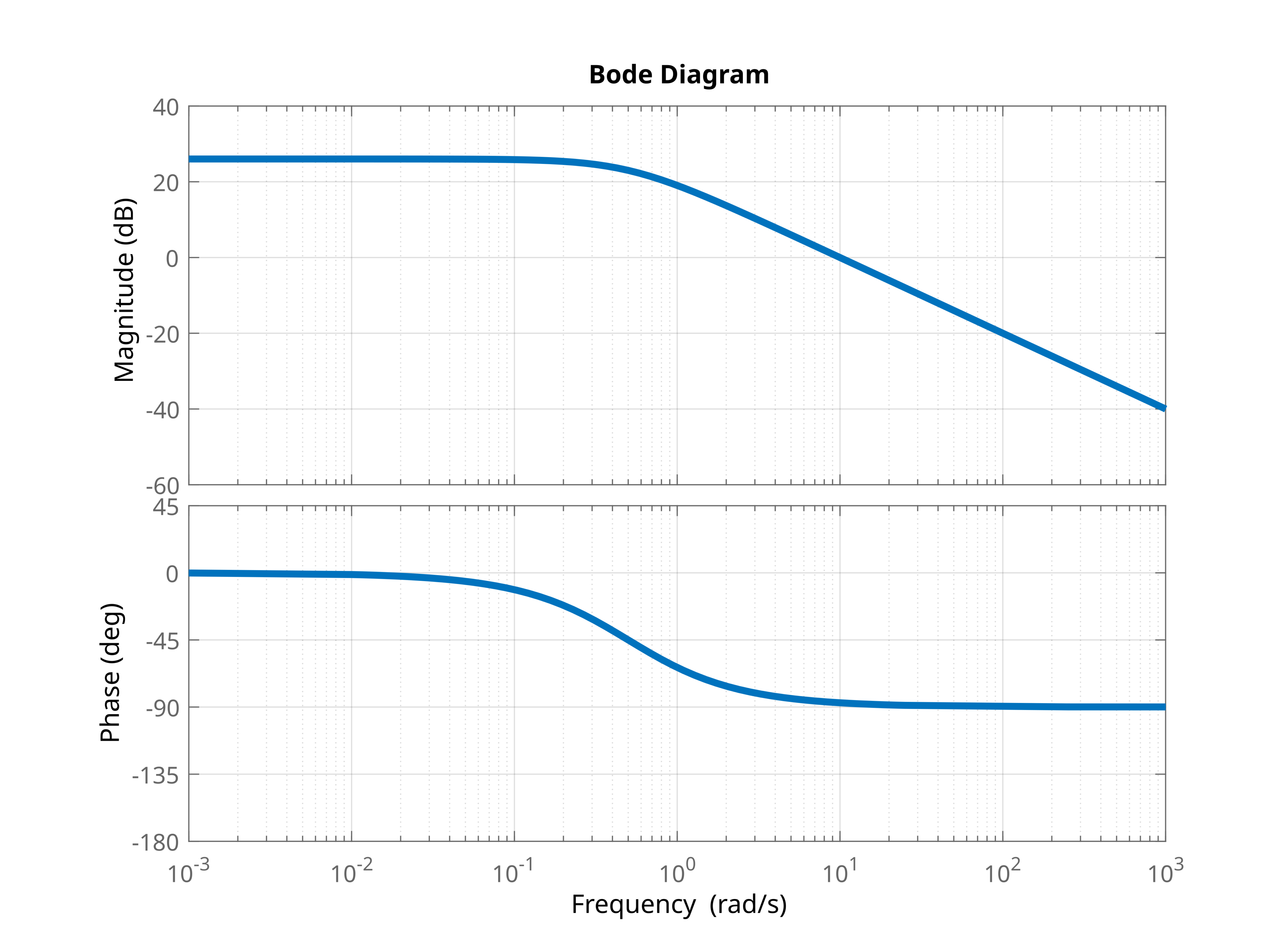
The Bode plot consists of two plots. The first plot (top plot) shows the log-magnitude function. The second plot (bottom plot) shows the phase function. On the horizontal axis, we plot the angular frequency in the logarithmic scale.

We transform the log-magnitude function as follows

(10) $\begin{align*}L=20\log_{10} \big( \frac{20}{\sqrt{1+4\omega^{2}}} \big)= 20\log_{10} \big( 20\big) -20\log_{10} \big( \sqrt{1+4\omega^{2}} \big)\end{align*}$

That is,

(11) $\begin{align*}L=L_{1}+L_{2}\end{align*}$

where

(12) $\begin{align*}L_{1}=20\log_{10} \big( 20\big)=26.02,\;\; L_{2}=-20\log_{10} \big( \sqrt{1+4\omega^{2}} \big)\end{align*}$

We first plot the function $L_{1}$ . This function is shown below

Figure 1: Log-magnitude plot of $L_{1}$ .

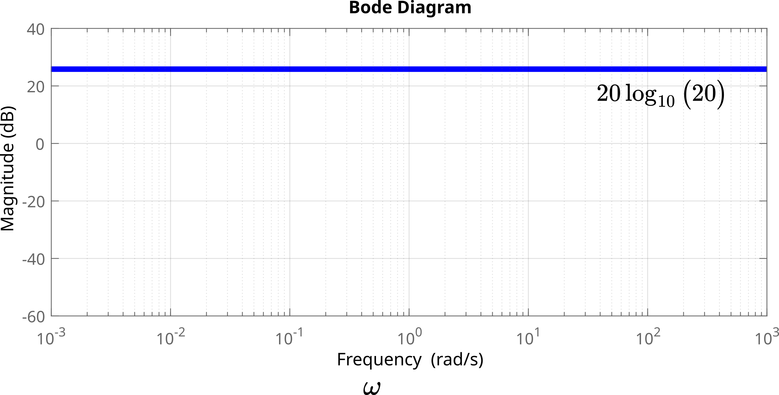Next, we plot $L_{2}$ . First, we construct the plot of $L_{2}$ by using asymptotes. Let us consider the general form of the first-order transfer function

(13) $\begin{align*}\frac{1}{1+Ts}\end{align*}$

This term is the general form of the expression that participates in our original transfer function. That is, the general form of

(14) $\begin{align*}\frac{1}{2s+1}\end{align*}$

where in our case, $T=2$ . The log-magnitude function of this transfer function is

(15) $\begin{align*}- 20 \log_{10}(\sqrt{1+T^{2}\omega^{2}})\end{align*}$

For $\omega T<<1$ we have

(16) $\begin{align*}-20 \log_{10}(\sqrt{1+T^{2}\omega^{2}}) \approx 0\end{align*}$

This is a horizontal straight line. On the other hand, for $\omega T>> 1$ we have

(17) $\begin{align*}-20 \log_{10}(\sqrt{1+T^{2}\omega^{2}}) \approx -20 \log_{10}(\omega T)\end{align*}$

This is a line with a slope of -20 dB per 10 times increase of the frequency $\omega$ . This slope is called a “-20 dB per decade” slope. A decade means a 10 times increase in the frequency. The frequency $\omega$ for which

(18) $\begin{align*}\omega T = 1,\;\; => \;\; \omega=\frac{1}{T}\end{align*}$

is called the break frequency or corner frequency. The point determined by this frequency is called the break point. The two asymptotes (16) and (17) meat at the break frequency. From another point of view, we can see the break frequency as the breakpoint from the horizontal asymptote to the slanted asymptote.

By using asymptotes, we plot the log-magnitude plot of $L_{2}$ . The break frequency is

(19) $\begin{align*}2 \omega =1,\;\; \omega=\frac{1}{2}=0.5\end{align*}$

The asymptotic approximation of $L_{2}$ is shown in the figure below.

Figure 3: The asymptotic approximation of $L_{2}$ .

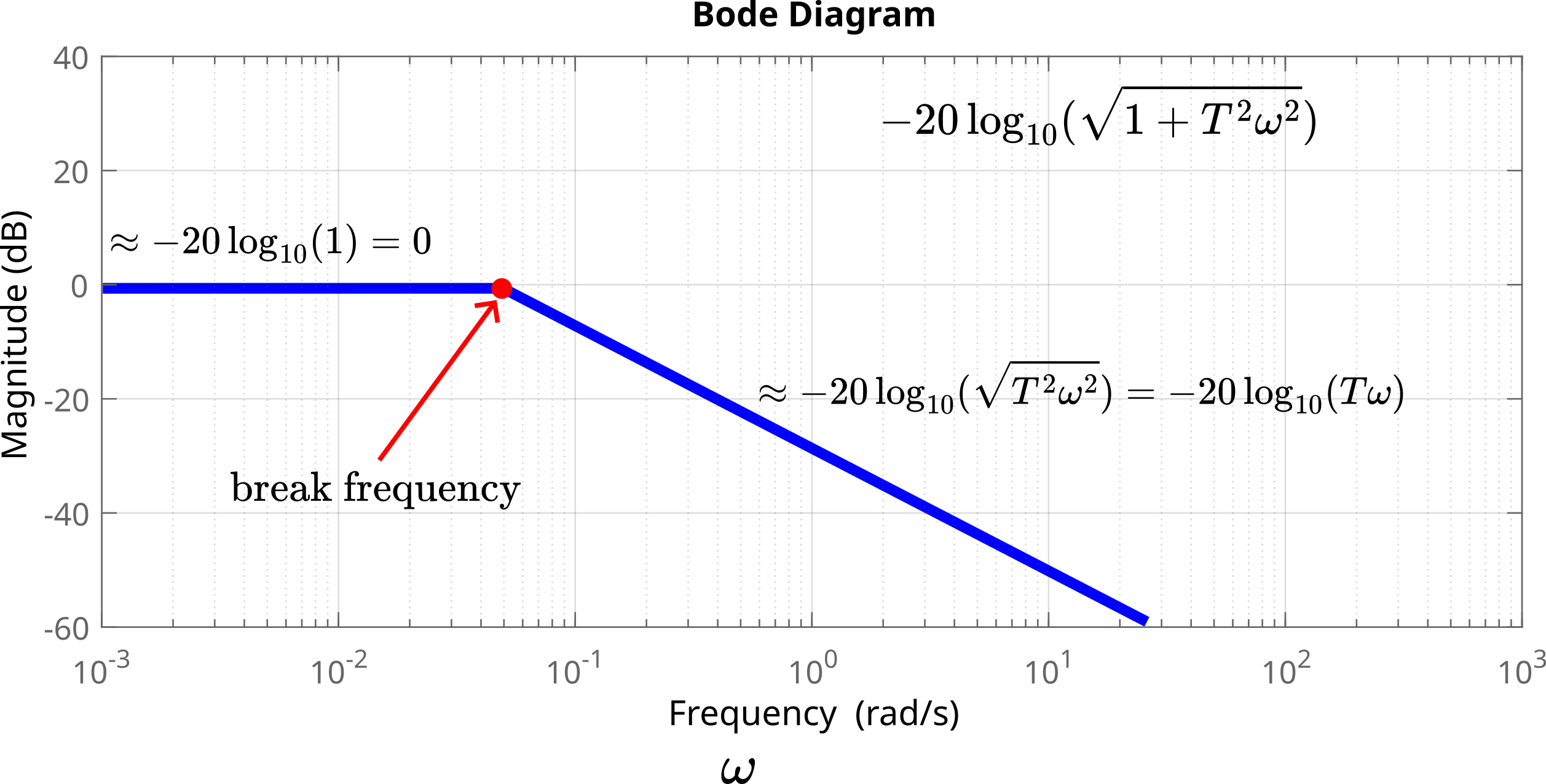At the break frequency, we have

(20) $\begin{align*}- 20 \log_{10}(\sqrt{2})\approx - 3.01 \;\; \text{dB}\end{align*}$

This means that at the break frequency point, we make an error of $- 3.01 \;\; \text{dB}$ if we approximate the log-magnitude plot of $L_{2}$ by linear asymptotes.

If we add $L_{1}$ and $L_{2}$ , we obtain the following diagram

Figure 4: Approximation of the log magnitude plot.

The log magnitude plot and asymptotic approximation are shown in the figure below.

Figure 5: Approximation and real log magnitude plot.

Finally, we need to sketch the phase plot. The phase is determined by the function

(21) $\begin{align*}\phi (\omega) =-\arctan(2\omega)\end{align*}$

When $\omega =0$ , we have $\phi=0$ . On the other hand, when $\omega = \infty$ , we have $\phi =-90$ deggres. On the other hand, when $\omega$ is equal to the break frequency, we have $\phi=-45$ . The phase function given below is a monotonically decreasing function of $\omega$ . We know this since $\arctan(2\omega)$ is a monotonically increasing function of $\omega$ . This means that $-\arctan(2\omega)$ is a monotonically decreasing function of $\omega$ . This leads us to the conclusion that the phase plot should look like this.