How to Design Parameter of Proportional-Integral Controllers by Using Routh-Hurwitz Stability Test – Fusion of Engineering, Control, Coding, Machine Learning, and Science

In this control engineering, robotics, and control theory tutorial, we explain how to design parameters of proportional-integral controllers by using the Routh-Hurwitz stability test. We explain how to determine the range of values of proportional and integral controllers that guarantee the asymptotic stability of the closed-loop system. Also, we simulate the dynamics of the closed-loop control system in MATLAB to verify the analytic computations. The method that is presented in this tutorial is a very simple method for finding ranges of control parameter values. You do not need MATLAB or advanced computation software to use this method, and you can compute the range of control parameters by hand.

The YouTube tutorial accompanying this webpage tutorial is given below.

Problem Formulation

The figure below shows a basic block diagram of a control system.

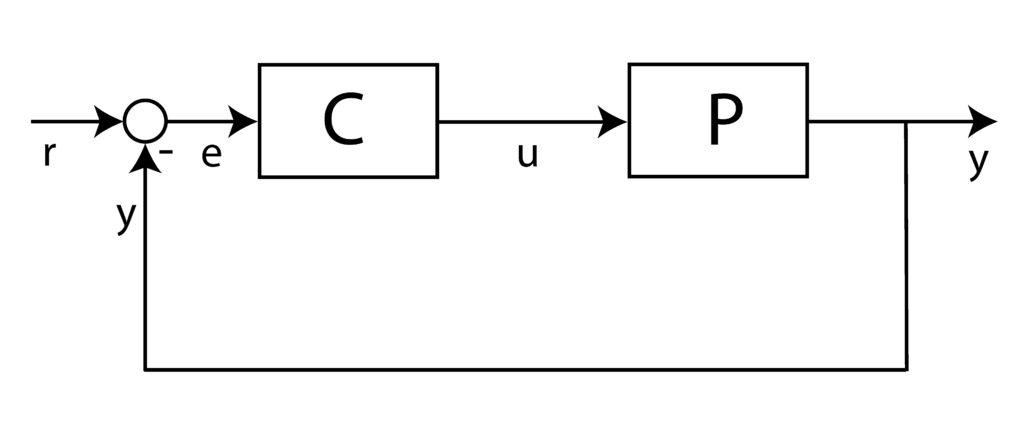
The block denoted by “P” denotes the plant. In the control engineering terminology, the plan is a dynamical system that we want to control. The block denoted by “C” is a controller or a control algorithm. The reference signal or the desired input signal is denoted by $r$ . The control signal which is the output of the control block and the input to the plant, is denoted by $u$ . The output of the system is denoted by $y$ . The output is the quantity measured by sensors. The control error $e$ is defined as the difference between the reference signal $r$ and the output of the system $y$

(1) $\begin{align*}e=r-y\end{align*}$

In this tutorial, we assume that the plant is mathematically described by the following differential equation:

(2) $\begin{align*} \ddot{y}+5\dot{y}+6y=u(t)\end{align*}$

where $\dot{y}$ and $\ddot{y}$ are the first and second-time derivatives of the system output $y$ . In this tutorial, we assumed a particular form of the model. However, everything explained in this tutorial can be generalized to second-order plants with arbitrary model coefficients as well as to higher-order plants.

The standard form of the Proportional-Integral (PI) control algorithm is given by this equation:

(3) $\begin{align*}u(t)=Ke(t)+K_{I}\int_{0}^{t} e(\tau) d\tau\end{align*}$

where $K$ is the proportional control gain or the proportional control parameter, and $K_{I}$ is the integral control gain or the integral control parameter.

Our goal is to select the control parameters $K$ and $K_{I}$ such that the closed-loop system in Fig. 1 is asymptotically stable.

Asymptotic stability of the closed loop system means that the control error $e$ will asymptotically approach zero as time approaches infinite. Zero control error means that the output of the system will asymptotically approach the reference signal $r$ .

How to Design Proportional and Integral Gains by Using the Routh-Hurwitz Stability Test

We solve the control problem by using the Routh-Hurwitz stability test. In our previous tutorial given here, we explained the basics of the Routh-Hurwitz stability test. Consequently, before reading this section of the tutorial, it is a good idea to read that tutorial in order to get yourself familiar with the Routh-Hurwitz stability test.

To solve our control design problem, we need to compute the transfer functions of the plan and controller. To compute the transfer function of the plant, we apply the Laplace transform to Eq. (2):

(4) $\begin{align*}(s^{2}+5s+6)Y(s)=U(s) \end{align*}$

where $s$ is the Laplace complex variable and the noation $Y(s)$ and $U(s)$ is used to denote the Laplace transforms of $y(t)$ and $u(t)$ , respectively. From this equation, we obtain the transfer function of the plant, denoted by $P(s)$ :

(5) $\begin{align*}P(s)=\frac{Y(s)}{U(s)}=\frac{1}{s^{2}+5s+6}\end{align*}$

On the other hand, by applying the Laplace transform to the control algorithm equation Eq.(3), we obtain

(6) $\begin{align*}U(s)=KE(s)+\frac{K_{I}}{s}E(s)\end{align*}$

where the notation $U(s)$ and $E(s)$ is used to denoted the Laplace transforms of $u(t)$ and $e(t)$ , respectively. From this equation, we obtain the transfer function of the controller:

(7) $\begin{align*}C(s)=\frac{U(s)}{E(s)}=K+\frac{K_{I}}{s}\end{align*}$

The transfer function of the closed-loop system is given by this equation:

(8) $\begin{align*}W(s)=\frac{Y(s)}{R(s)}\end{align*}$

where $R(s)$ is the Laplace transform of $r(t)$ . From the block diagram shown in Fig. 1, we obtain

(9) $\begin{align*}Y(s)=P(s)C(s)E(s)\end{align*}$

The error in the complex Laplace domain is defined by this equation

(10) $\begin{align*}E(s)=R(s)-Y(s)\end{align*}$

By substituting Eq.(10) in Eq.(9), we obtain the following equation

(11) $\begin{align*}Y(s)=P(s)C(s)R(s)-P(s)C(s)Y(s) \end{align*}$

From this equation, we further obtain

(12) $\begin{align*}(1+P(s)C(s))Y(s)=P(s)C(s)R(s)\end{align*}$

and this equation produces

(13) $\begin{align*}W(s)=\frac{Y(s)}{R(s)}=\frac{P(s)C(s)}{1+P(s)C(s)}\end{align*}$

The equation Eq.(13) immediately gives us the characteristic polynomial of the closed-loop system:

(14) $\begin{align*}1+P(s)C(s)=0\end{align*}$

Next, we substitute the values for $P(s)$ and $C(s)$ , which are defined in Eqs. (5) and (6), in Eq. (14). After simple algebraic transformations, we obtain the following polynomial

(15) $\begin{align*}s^{3}+5s^2+(6+K)s+K_{I}=0\end{align*}$

From the Routh-Hurwitz stability test, we know that the first necessary condition for asymptotic stability is that all the coefficients in the characteristic polynomial have to be positive. The equivalent statement is that all the coefficients have to have the same sign. From this condition, we have

(16) $\begin{align*}K_{I}>0,\;\;\; 6+K>0 \end{align*}$

Next, we need to determine the sufficient conditions on the range of values of $K_{I}$ and $K$ that will guarantee the asymptotic stability of the closed loop system. The Routh array (Routh-Hurtwitz array) for the characteristic polynomial given in Eq. (15) is

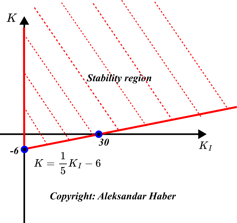
(17) $\begin{align*} \begin{matrix} 1 & & 6+K \\ 5 & & K_{I} \\ \frac{30+5K-K_{I}}{5} & & 0 \\ K_{I} & & 0 \end{matrix}\end{align*}$

According to the Routh-Hurwitz stability test, all the coefficients in the first column of the Routh array have to be positive in order to guarantee asymptotic stability. That is, if

(18) $\begin{align*}K_{I}>0,\;\;\;\; K>\frac{K_{I}}{5}-6\end{align*}$

then the system is asymptotically stable. The system of inequalities in Eq. (18) defines a region in the K_{I}-K plane that is illustrated in the figure shown below.

The region of control parameter values that guarantee the asymptotic stability of the system.

Next, we need to verify our analytic computations by simulating the closed-loop system response in MATLAB. The MATLAB script given below defines the controller and plant, and simulates the closed-loop response of the system.

s = tf('s')

Ki= 1
% this is the boundary: K= (1/5)*Ki-6, stability region is Ki>0 and K> (1/5)*Ki-6 
K= (1/5)*Ki-6+0.21

P=1/(s^2+5*s+6)
C=K+Ki/s

% closed-loop transfer function
W=P*C/(1+P*C)

pole(W)

step(W)

X0=randn(6,1)

initial(ss(W),X0)

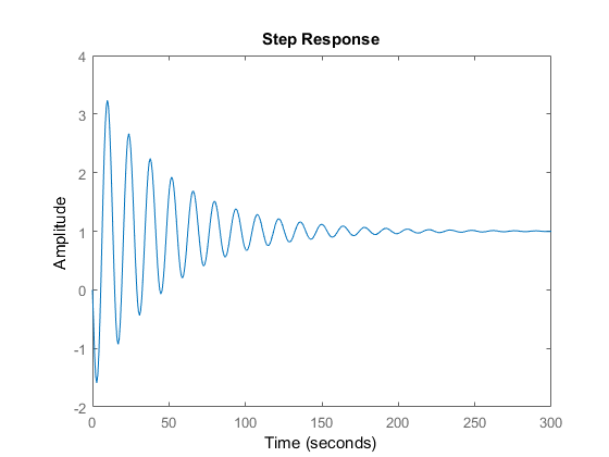
The step response of the closed loop system is given below.

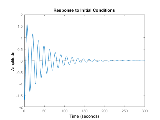
Figure 2: The step response of the closed loop system.

The response of the closed-loop system to a non-zero initial state is given below.

Problem Formulation

How to Design Proportional and Integral Gains by Using the Routh-Hurwitz Stability Test

admin

You might also like

Control Systems Lecture: Simulation of linear ordinary differential equations using Python and state-space modeling

Quadratic Forms, Positive Definite, Negative Definite, and Semi-Definite Matrices

Correct Explanation of State Observers for State Estimation of State-Space Models with Python Simulations