Calibration of Thermistors – Conversion of Readings Into Temperature – Fusion of Engineering, Control, Coding, Machine Learning, and Science

In this post, we explain how to convert thermistor readings into temperatures. We use a least-squares method and we give a MATLAB code. We explain the complete procedure of how to set up a least-squares problem and how to solve it. We also give an example that is based on industrial thermistor. The video accompanying this post, is given below:

In its essence, a thermistor is basically a resistor whose resistance is highly dependent on its temperature. Consequently, we can use them as temperature sensors. Let us assume that we have installed a thermistor and that we have implemented a data acquisition system that is able to give us voltage or current or resistance of the thermistor. For example, if know the voltage and the current, we can compute the resistance using Ohm’s law.

Now, the problem is to convert the computed resistance to temperature. That is we need a calibration curve or a set of points in a resistance-temperature coordinate system that can be used to fit the calibration curve. Usually, a thermistor manufacturer will provide us data for fitting the calibration curve. If we do not have these points, then we can experimentally obtain such points as follows. For example, we can use another temperature sensor (in the sequel we refer to this sensor as a “second sensor”). Assuming that it is accurate, we can place this sensor very close to the thermistor. Then we can obtain a resistance of the thermistor. The temperature measured by the second sensor and the resistance of the thermistor represent a single point on a graph. By repeating this procedure for different values of temperature, we can obtain other points. For example, we can place the second sensor and the thermistor on top of a hot plate whose temperature can be regulated.

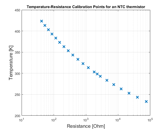
To demonstrate how to fit a calibration curve, we will use real-world data. On this website, you can find a set of points (resistance-temperature) for an industrial thermistor ACC101, supplied by Ametherm. This thermistor is of the NTC type, where NTC stands for Negative Temperature Coefficient. That is, for this thermistor type, as the temperature increases, the resistance increases.

Using the data provided on the website, we obtain the following calibration points.

Next, we explain the calibration procedure. In order to fit a function, or better to say in order to fit function parameters that explain the calibration points, we need to have some a priori knowledge. It turns out that the mathematical relation between temperature and resistance for NTC thermistors has extensively been studied. The relation is described by the Steinhart-Hart equation:

(1) $\begin{align*}\frac{1}{T}=a+b \cdot ln(R)+ c \cdot \Big( ln(R) \Big)^{3}\end{align*}$

where $a,b$ and $c$ are parameters that need to be estimated, $R$ is the resistance measured in $[\Omega]$ , $T$ is temperature (absolute temperature) measured in $[K]$ , and $ln(\cdot)$ is a natural logarithm.

The problem of estimating the parameters $a,b$ and $c$ , can be formulated as follows. Given a set of $N$ points $\{ (T_{1},R_{1}),(T_{2},R_{2}),\ldots, (T_{N},R_{N}) \}$ , estimate the constants $a,b$ and $c$ in (1).

To solve this problem, we use a least-squares method. First, we introduce new variables.

(2) $\begin{align*}y=\frac{1}{T},\;\; x=ln(R)\end{align*}$

Consequently, we can transform (1), as follows

(3) $\begin{align*}y=a+bx+cx^{3}\end{align*}$

The last equation, can be written in the vector notation

(4) $\begin{align*}y=\begin{bmatrix}1 & x & x^{3} \end{bmatrix}\begin{bmatrix}a\\ b \\c \end{bmatrix}\end{align*}$

By substituting $N$ measurement points in (4), and by writting the resulting equation in a matrix form, we obtain

(5) $\begin{align*}\underbrace{\begin{bmatrix}y_{1} \\ y_{2} \\ \vdots \\ y_{N} \end{bmatrix}}_{\mathbf{z}}=\underbrace{\begin{bmatrix}1 & x_{1} & x_{1}^{3} \\ 1 & x_{2} & x_{2}^{3} \\ \vdots & \vdots & \vdots \\ 1 & x_{N} & x_{N}^{3} \end{bmatrix}}_{A}\underbrace{\begin{bmatrix} a \\ b \\ c \end{bmatrix}}_{\boldsymbol{\theta}}\end{align*}$

where $y_{i}=1/T_{i}$ , and $x_{i}=ln(R_{i})$ . We can compactly write (5) as follows:

(6) $\begin{align*}\mathbf{z}=A\boldsymbol{\theta}\end{align*}$

where $\mathbf{z}\in \mathbb{R}^{N}$ , $A\in \mathbb{R}^{N\times 3 }$ , and $\boldsymbol{\theta}\in \mathbb{R}^{3}$ .
The vector of parameters $\boldsymbol{\theta}$ , can be estimated by solving the following least-squares problem

(7) $\begin{align*}\min_{\boldsymbol{\theta}} \left\|\mathbf{z}-A\boldsymbol{\theta} \right\|_{2}^{2}\end{align*}$

Assuming that $N\ge 3$ and that $A$ is of full rank, the solution (7) is given by

(8) $\begin{align*}\hat{\boldsymbol{\theta}}=\Big(A^{T}A \Big)^{-1}A^{T}\mathbf{z}\end{align*}$

where

(9) $\begin{align*}\hat{\boldsymbol{\theta}}=\begin{bmatrix} \hat{a} \\ \hat{b} \\ \hat{c} \end{bmatrix}\end{align*}$

and where $\hat{a},\hat{b}$ , and $\hat{c}$ are the estimates of the parameters $a,b$ , and $c$ . Once we have estimated the parameters, we can subsitute them into the equation for temperature. From (1), we have

(10) $\begin{align*}T=\frac{1}{\hat{a}+\hat{b}\cdot ln(R)+ \hat{c}\cdot\Big( ln(R) \Big)^{3}}\end{align*}$

The MATLAB code for computing the parameter is given below

clear,pack,clc
% data taken from: https://www.digikey.com/en/products/detail/ametherm/ACC101/5967501?s=N4IgTCBcDaIIYFsCmAXAFkgTggBHAxvgIwAMRO6WCAlgM4oD2mIAugL5A
R = [75780, 39860, 21860, 12460, 7352.8, 4481.5, 2812.8, 2252, 1814.4, 1199.6, 811.40, 560.30, 394.55, 282.63, 206.13, 152.75, 114.92, 87.671, 67.77, 52.983, 41.881];
T =273.15+[-40,-30,-20,-10,0,10,20,25,30,40,50,60,70,80,90,100,110,120,130,140,150];

%T=T(6:end)
%R=R(6:end)

plot(R,T)

% getting the calibration constants:a,b,c
% 1/T=a+b*log(R)+c*(log(R))^3
% y=a+b*x+c*x^3
% x=log(R)
% y=1/T
% Steinhart–Hart equation
%https://en.wikipedia.org/wiki/Thermistor

x=log(R)
z=1./T
s1=numel(R)

for i=1:s1
    A(i,1)=1
    A(i,2)=x(i)
    A(i,3)=x(i)^3
end

parameters=inv(A'*A)*A'*z'

The estimated parameters are $\hat{a}= 0.0015$ , $\hat{b}=2.3814e-04$ , and $\hat{c}=1.0188e-07$ . These values are in agreement with the results reported in the Wikipedia page.

Here a few comments are in order. If you know the expected temperature change, then better results are achieved by using the data points that are in the expected temperature range. In the example shown above, we have used a relatively large temperature range that might not produce very accurate results if the temperature range is for example in the range [20,30] Celsius.

admin

You might also like

Eigen C++ Matrix Library Tutorial – Saving and Loading Data In and From CSV Files

Easy-to-Understand Explanation of Controllable Canonical Form – (also known as Reachable or Control Canonical form)

Solve Ordinary Differential Equations in Python by Using odeint() Function