7. Accurately Compute Relative Strength Index (RSI) of Stock Time-Series in Python – Fusion of Engineering, Control, Coding, Machine Learning, and Science

In this tutorial, we will learn how to compute the Relative Strength Index (RSI) of stock time-series in Python. This indicator can be used to develop a trading strategy. The video accompanying this post is given here:

I realized that there are many websites that provide incomplete information on how this indicator is calculated. Furthermore, there are many websites that use inaccurate methods to compute this important indicator. Consequently, I had to consult the original work of J. Welles Wilder Jr. in which the RSI is defined. The name of the book is “New Concepts in Technical Trading Systems” and it was published in 1978. The Wikipedia page of J. Welles Wilder Jr says that he has a mechanical engineering background. To me, this does not come as a surprise since from my personal experience I know that mechanical engineers can apply their knowledge and developed intuition to various real-life problems.

So let us see how the RSI is being defined according to “New Concepts in Technical Trading Systems” (page 65, Section 6). Let $\{ x_{k}, k=0,1,2,\ldots \}$ be a stock closing-price time series. Let $N$ be a period for the computation of the RSI indicator.

Step 1: Compute the price differences. That is, first we compute $\Delta {x}_{1}=x_{1}-x_{0}$ , $\Delta {x}_{2}=x_{2}-x_{1}$ , $\Delta {x}_{3}=x_{3}-x_{2}$ , etc. In the general case, the price difference is given by $\Delta {x}_{i}={x}_{i}-{x}_{i-1}$ .

Step 2: Compute the initial values for the RSI recuirsions. Let $\{\Delta x_{i}^{+} \}$ be time-series defined for $i=1,2,\ldots, N$ as follows:

(1) $\begin{align*}& \Delta x_{i}^{+} = \Delta x_{i}, \;\; \text{if}\;\; \Delta x_{i}\ge 0 \\& \Delta x_{i}^{+} = 0, \;\; \text{if}\;\; \Delta x_{i} < 0\end{align*}$

Similarly, let $\{\Delta x_{i}^{-} \}$ be time-series defined for $i=1,2,\ldots, N$ as follows:

(2) $\begin{align*}& \Delta x_{i}^{-} = |\Delta x_{i}|, \;\; \text{if}\;\; \Delta x_{i}\le 0 \\& \Delta x_{i}^{-} = 0, \;\; \text{if}\;\; \Delta x_{i} > 0\end{align*}$

For example, if $N=3$ , and $\Delta {x}_{1}=1.2$ , $\Delta {x}_{2}=-0.1$ , and $\Delta {x}_{3}=-0.5$ , we have:

$\Delta {x}_{1}^{+}=1.2$ , $\Delta {x}_{2}^{+}=0$ , and $\Delta {x}_{3}^{+}=0$

and

$\Delta {x}_{1}^{-}=0$ , $\Delta {x}_{2}^{-}=0.1$ , and $\Delta {x}_{3}^{-}=0.5$

Next, we compute the averages of the time series $\{\Delta x_{i}^{+} \}$ and $\{\Delta x_{i}^{-} \}$ :

(3) $\begin{align*} \overline{\Delta x}^{+}=\frac{\sum_{i=1}^{N} \Delta x_{i}^{+} }{N}\end{align*}$

and

(4) $\begin{align*}\overline{\Delta x}^{-}=\frac{\sum_{i=1}^{N} \Delta x_{i}^{-} }{N}\end{align*}$

The relative strength is then computed as

(5) $\begin{align*}w=\frac{\overline{\Delta x}^{+}}{\overline{\Delta x}^{-}}\end{align*}$

where $w$ is the relative strength. Then, the RSI is computed as

(6) $\begin{align*}q=100 - \frac{100}{1+w}\end{align*}$

where $q$ is used to denote the RSI.

Step 3. First, we initialize the following variables:

(7) $\begin{align*}& \overline{\Delta x}^{+}_{N}=\overline{\Delta x}^{+} \\& \overline{\Delta x}^{-}_{N}=\overline{\Delta x}^{-} \\& w_{N}=w \\& q_{N} = q\end{align*}$

where $\overline{\Delta x}^{+}$ , $\overline{\Delta x}^{-}$ , $w$ and $q$ are computed in the initial step 2 explained above.

For $k=N,N+1,N+2,\ldots$ , recursively compute

(8) $\begin{align*}\overline{\Delta x}^{+}_{k+1}=\frac{N-1}{N}\overline{\Delta x}^{+}_{k}+\frac{1}{N}\Delta x^{+}_{k+1} \\\overline{\Delta x}^{-}_{k+1}=\frac{N-1}{N}\overline{\Delta x}^{-}_{k}+\frac{1}{N}\Delta x^{-}_{k+1}\end{align*}$

where $\overline{\Delta x}^{+}_{k}$ and $\overline{\Delta x}^{-}_{k}$ are the averages at the time steps $k=N,N+1,N+2,\ldots$ , and $\Delta x^{+}_{k+1}$ and $\Delta x^{-}_{k+1}$ are the price differences that are computed according to (1) and (2). Once we have updated the averages, we can compute the RSI as follows

(9) $\begin{align*}& w_{k+1}=\frac{\overline{\Delta x}^{+}_{k+1}}{\overline{\Delta x}^{-}_{k+1}} \\& q_{k+1}= 100 - \frac{100}{1+w_{k+1}}\end{align*}$

The above-explained computational steps, produce a time series of the RSI: $q_{N},q_{N+1},q_{N+1},\ldots$ .

The code for computing the RSI is given below. We download the SPY stock (ETF) prices and we plot the closing price and the computed RSI.

# -*- coding: utf-8 -*-
"""
Compute Relative Strength Index (RSI) of stock time series in Python 

Source: 

 “New Concepts in Technical Trading Systems” (page 65, Section 6). 
by J. Welles Wilder Jr

Author:
    Aleksandar Haber

Date: January 25, 2021
Some parts of this code are inspired by the following sources:
    
-- https://www.datacamp.com/community/tutorials/pickle-python-tutorial
-- Pandas help: https://pandas.pydata.org/pandas-docs/stable/reference/api/pandas.DataFrame.ewm.html
-- "Learn Algorithmic Trading: Build and deploy algorithmic trading systems and strategies
using Python and advanced data analysis", by Sebastien Donadio and Sourav Ghosh


"""

# standard imports
import pandas as pd 
import numpy as np
import matplotlib.pyplot as plt
# used to download the stock prices
import pandas_datareader as pdr


# define the period parameter for RSI

period_RSI=14

# define the dates for downloading the data, the date difference should be 
# larger than the RSI period
startDate= '2020-8-1'
endDate= '2021-2-3'


stock_symbol='SPY'

# download the data from Yahoo 

data = pdr.get_data_yahoo(stock_symbol,start=startDate,end=endDate)


# inspect the data

data.head()

data['Close'].plot()

# isolate the closing price
closingPrice = data['Close']


differencePrice = data['Close'].diff()
differencePriceValues=differencePrice.values

positive_differences=0
negative_differences=0
current_average_positive=0
current_average_negative=0
price_index=0
RSI=[]

for difference in differencePriceValues[1:]:
    
    if difference>0:
        positive_difference=difference
        negative_difference=0                
    if difference<0:
        negative_difference=np.abs(difference)
        positive_difference=0
    if difference==0:
        negative_difference=0
        positive_difference=0
    
    # this if block is used to initialize the averages
    if (price_index<period_RSI):
        
        current_average_positive=current_average_positive+(1/period_RSI)*positive_difference
        current_average_negative=current_average_negative+(1/period_RSI)*negative_difference
              
        if(price_index==(period_RSI-1)):
            #safeguard against current_average_negative=0
            if current_average_negative!=0:
                RSI.append(100 - 100/(1+(current_average_positive/current_average_negative)))           
            else:
                RSI.append(100)
    # this is executed for the time steps > period_RSI, the averages are updated recursively        
    else:
        
        current_average_positive=((period_RSI-1)*current_average_positive+positive_difference)/(period_RSI)
        current_average_negative=((period_RSI-1)*current_average_negative+negative_difference)/(period_RSI)
        
        #safeguard against current_average_negative=0
        if current_average_negative!=0:
            RSI.append(100 - 100/(1+(current_average_positive/current_average_negative)))   
        else:
            RSI.append(100)
            
    price_index=price_index+1    
        
#create the RSI time series
RSI_series=pd.Series(data=RSI,index=data['Close'].index[period_RSI:])

# create the 30 and 70 limit lines

num_entries=RSI_series.values.size

line30=num_entries*[30]
line70=num_entries*[70]

# create the Pandas dataframe with 30 and 70 line limits 
lines30_70=pd.DataFrame({'30 limit': line30, '70 limit': line70},index=RSI_series.index)

    
# plot RSI and prices on the same graph

with plt.style.context('ggplot'):
    import matplotlib
    font = { 'weight' : 'bold',
        'size'   : 14}
    matplotlib.rc('font', **font)
    fig = plt.figure(figsize=(20,20))
    ax1=fig.add_subplot(211, ylabel='Stock price $')
    data['Adj Close'].iloc[period_RSI:].plot(ax=ax1,color='r',lw=3,label='Close price',legend=True)
    ax2=fig.add_subplot(212, ylabel='RSI')
    RSI_series.plot(ax=ax2,color='k',lw=2,label='RSI',legend=True)
    lines30_70['30 limit'].plot(ax=ax2, color='r', lw=4, linestyle='--')
    lines30_70['70 limit'].plot(ax=ax2, color='r', lw=4, linestyle='--')
    plt.savefig('RSI.png')
    plt.show()

This code produces the following diagrams.

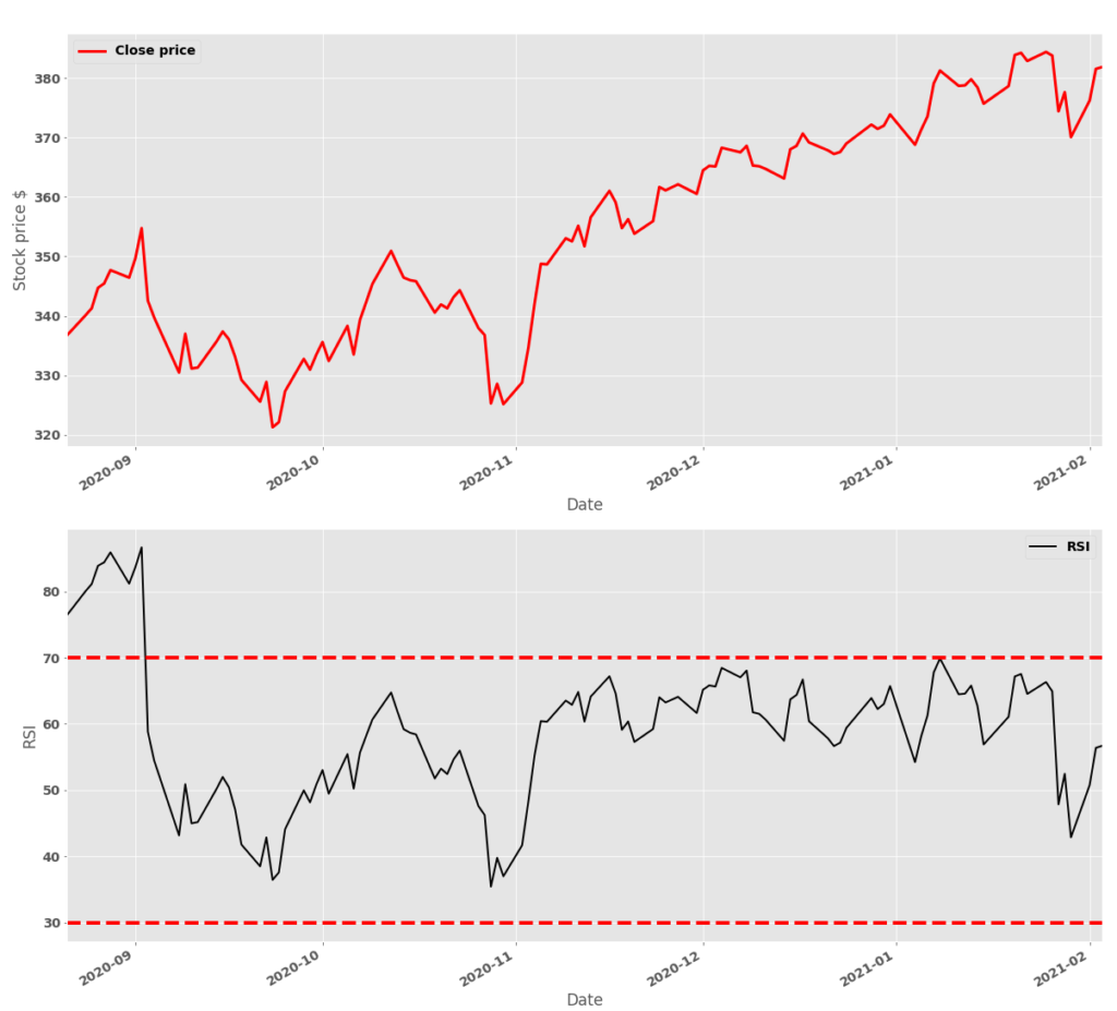
Figure 1: Top: SPY closing price. Bottom: RSI of the closing price. The red dashed line represent the 30 and 70 limits.

Figure 1 shows the closing price and the computed RSI. We also plot the 30 and 70 limits that are used as oversold/overbought limits.

admin

You might also like

Calibration and noise reduction of distance sensors (SHARP 2Y0A21 infrared sensors)

ABB Robot Tutorial: Defining Tool Frames and Basic Modeling in ABB RobotStudio

Deformation, Strain, and Hooke’s law