Multi-armed Bandit Problem: Epsilon-Greedy Action Value Methods With Python Codes and Implementation – Fusion of Engineering, Control, Coding, Machine Learning, and Science

In this post, we explain the multi-armed bandit problem. We explain how to approximately (heuristically) solve this problem, by using an epsilon-greedy action value method and how to implement the solution in Python. The YouTube video accompanying this post is given below.

The GitHub pages with all the codes is given here.

Motivational Examples

In the sequel, we introduce several examples that explain the multi-armed bandit problem.

EXAMPLE 1: Doctor who wants to select the most effective treatment. Let us imagine that we are a doctor who wants to come up with the most effective treatment for sick patients. Let us assume that we have 3 possible treatments that we can select. Let these treatments be called actions. Let us assume that every time we apply the same treatment (action), we obtain a different health outcome quantified by a numerical value. The health outcome can be for example the percentage of the recovery of the patient from the disease, or some numerical measure that measures the presence of a virus or cancer in the body of the patient. The variability of the same outcome can be due to many factors. For example, every patient is different, and every person will most likely react differently (even slightly) to the same treatment. Even if we apply the same treatment (action) to the same patient over a time interval, we will most likely obtain different results. If we have enough data, for every action, we can construct a probability distribution that will quantify the effectiveness of the treatment. We call the numerical value of the outcome the reward. The higher the reward, the more effective the treatment is for a particular patient. Assuming that we have enough data, we can construct the probability distributions for every action that are shown in Fig. 1.

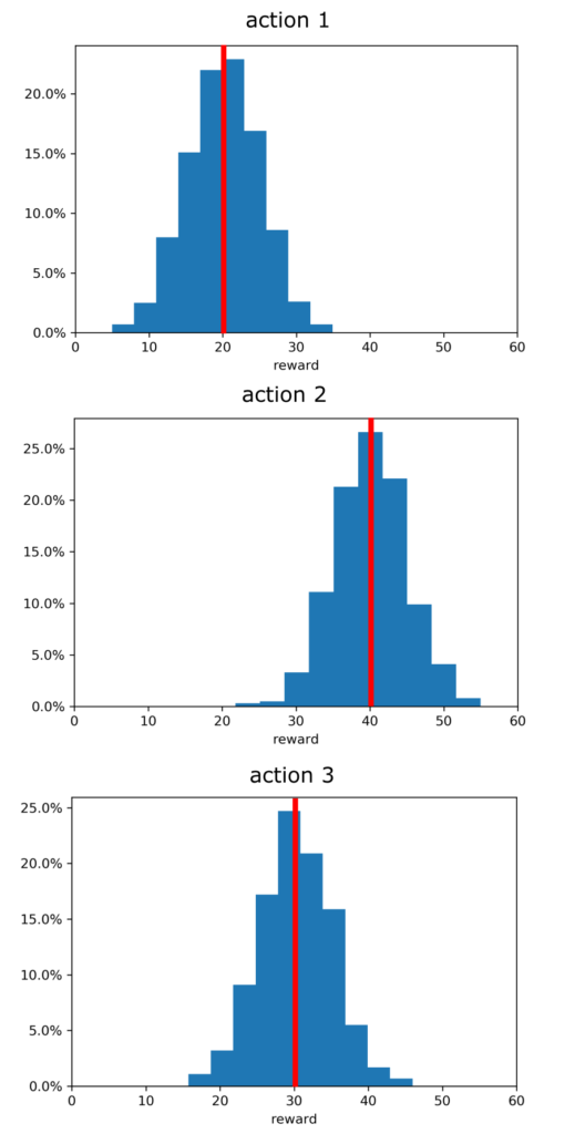
Figure 1: Empirical probability distributions of rewards for different actions. The red lines denote the empirical means.

If we would know the distributions shown in Fig.1, then our choice would be relatively easy. The most “rewarding” action is action 2, since “on average” it gives the highest reward. However, we often do not know these distributions a priori (that is, before a large number of actions are taken and outcomes are observed). A priori is just a fancy word for prior knowledge or advance knowledge before something has happened. The multi-armed bandit problem is to design a sequence of actions that will maximize the expected total reward over some time period. Also, in the literature, this problem is also defined as the problem that aims at finding a sequence of actions that will maximize the sum of rewards over a certain time period.

EXAMPLE 2: Casino Gambler. The name of the multi-armed bandit problem is motivated by this problem. Consider a gambler who has a choice to play three slot machines. A slot machine is usually called a one-armed bandit. The slot machine is operated by a single arm (also called a lever). When we pull an arm of the machine, we obtain a reward. Our gambler needs to figure out how to play these 3 machines such that he or she maximizes the sum of rewards over a time period. We assume that every machine produces a different reward outcome every time a lever is pulled (arm is pulled). That is, to every machine we can associate a probability distribution that describes the probability of obtaining a certain reward. We assume that our gambler does not know a priori these distributions, otherwise, his task would be easy. So, the multi-armed bandit problem, in this case, is to design a sequence of actions (what slot machines to play at certain time steps) in order to maximize the total expected reward over a certain time period.

Solution of the Multi-Armed Bandit Problem

Now that we have introduced the multi-armed bandit problem through examples let us see how to tackle this problem. Again, let us repeat our problem once more:

The multi-armed bandit problem is to design a sequence of actions that will maximize the expected total reward over some time period.

To solve this problem, instead of dealing with distributions caused by certain actions, we need to deal with one number that will somehow quantify the distribution. Every distribution has an expected or a mean value. Consequently, expected or mean values are a good choice for tackling this problem. Let us first introduce a few definitions.

The number of arms is denoted by $N$ .
The action is denoted by $a_{i}$ , where $i=1,2,\ldots, N$ . The action $a_{i}$ is actually the selection of the arms $i$ .
The action selected at the time step $k$ is denoted by $A_{k}$ . Note that $A_{k}$ is a random variable.
The action $A_{k}$ can take different numerical values $a_{1}, a_{2},..,\ldots,a_{N}$ . A numerical value of the action $i$ is denoted by $a_{i}$ .
Every action $A_{k}$ at the time step $k$ , produces a reward that we denote by $R_{k}$ . Note that $R_{k}$ is a random variable.
The expected or the mean reward of the action we take is referred to as the value of that action. Mathematically speaking, the value is defined by
(1) $\begin{align*}v_{i}=v(a_{i})=E[R_{k}|A_{k}=a_{i}]\end{align*}$

where $v_{i}=v(a_{i})$ is the value of the action $a_{i}$ . In the case of Fig.1, the values are $v_{1}=20$ (action 1), $v_{2}=40$ , and $v_{3}=30$ .

Now, if we would know in advance the values of actions $v_{i}$ , $i=1,2,3,\ldots, N$ , our task would be completed: we would simply select the action that produces the largest value!

However, we do not know in advance the values of actions. Consequently, we have to design an algorithm that will learn the most appropriate actions that will minimize the sum of rewards over time.

For that purpose, we will use an action value method. The action values method aims at estimating the values of actions and using these estimates to take proper actions that will maximize the sum or rewards.

The story goes like this. At every time step $k$ we can select any of the actions $a_{i}$ . The action that is selected at the time step is denoted by $A_{k}$ . The reward produced by this action is $R_{k}$ . So, as the discrete-time $k$ progresses, we will obtain a sequence of actions $A_{1}, A_{2},\ldots$ , and a sequence of produced rewards $R_{1},R_{2},\ldots$ . From this data, we want to estimate a value of every action, that is denoted by $v_{i}=v(a_{i})$ . We can estimate these values at the time step $k$ , as follows

(2) $\begin{align*}\hat{v}_{i,k}=\hat{v}_{k}(a_{i})=\frac{\sum_{j=1}^{k-1} R_{i,j}}{n_{i,k}}\end{align*}$

where

$R_{i,j}$ is the reward produced by the action $a_{i}$ at the time step $j$ .
if the action $a_{i}$ is not selected at the time step $j$ , $j=1,2,\ldots, k-1$ , then $R_{i,j}=0$ in the above sum $\sum_{j=1}^{k-1} R_{j}$ .
$n_{i,k}$ is the number of times the action $a_{i}$ is selected before the step $k$ . If $n_{i,k}$ is zero, then we simply set $\hat{v}_{i,k}$ to zero to avoid division with zero issues.

To explain (4), consider the following case. Let us assume that $k=5$ , and that we have $A_{1}=a_{1}$ , $A_{2}=a_{1}$ , $A_{3}=a_{2}$ , and $A_{4}=a_{1}$ . Then, let us assume that $R_{1}=1$ , $R_{2}=2$ , $R_{3}=5$ , $R_{4}=4$ . This implies, $R_{1,1}=1$ , $R_{1,2}=2$ , $R_{1,3}=0$ , and $R_{1,4}=4$ . Similarly, $R_{2,1}=0$ , $R_{2,2}=0$ , $R_{2,3}=5$ , and $R_{2,4}=0$ . Then, since action $a_{1}$ is selected 3 times, we have $n_{1,5}=3$ . Similarly, since the action $a_{2}$ is selected one time before $k$ , we have $n_{2,5}=1$ . Consequently, we have

(3) $\begin{align*}& \hat{v}_{1,5}=\frac{1+2+0+4}{3}=\frac{7}{3}=\approx 2.33 \\& \hat{v}_{2,5}=\frac{0+0+5+0}{1}=\frac{5}{1}=5\end{align*}$

In practice, we usually do not use the average (4) to estimate action values. This is because we need to store all rewards obtained before the time step $k$ in order to compute the average. As the time step can be extremely large, it is computationally infeasible to store all the rewards. Instead, we use a recursive formula for averages. This formula can be derived as follows. Let us simplify the notation, and let us focus on the following average

(4) $\begin{align*}\hat{v}_{k} & =\frac{\sum_{j=1}^{k-1}R_{j}}{k-1} \\& = \frac{1}{k-1}(R_{k-1}+\sum_{j=1}^{k-2}R_{j}) \\& = \frac{1}{k-1}(R_{k-1}+\frac{k-2}{k-2}\sum_{j=1}^{k-2}R_{j}) \\& =\frac{1}{k-1}(R_{k-1} + (k-2) \hat{v}_{k-1}) \\& =\frac{1}{k-1}(R_{k-1} + (k-1)\hat{v}_{k-1}-\hat{v}_{k-1}) \\& = \hat{v}_{k-1}+\frac{1}{k-1}(R_{k-1}-\hat{v}_{k-1})\end{align*}$

Consequently, we obtain the following formula for the update of the average

(5) $\begin{align*}\hat{v}_{k} =\hat{v}_{k-1}+\frac{1}{k-1}(R_{k-1}-\hat{v}_{k-1})\end{align*}$

We will use (5) in the Python code that we will explain in the sequel to compute the averages.

At a first glance, it might be logical to base our decision on selecting the particular action $a_{i}$ at the time step $k$ , on the following criterion

(6) $\begin{align*}A_{k}=\text{max}_{a_{i}} \{ \hat{v}_{1,k},\hat{v}_{2,k},\ldots, \hat{v}_{N,k} \}\end{align*}$

That is, we can select the action $a_{j}$ that corresponds to the max value of the action value estimates at the discrete time step $k$ . This approach is often referred to as the greedy approach. That is, at every time step $k$ , we are greedy, and we want to select the action that maximizes the past estimate of the action value. This step is also the exploitation step. We are basically exploiting our past knowledge to gain future gain. However, there are several issues with this approach. One of the issues is that we rely too much on our past experience for making decisions. If our past experience is limited, then our future decisions will be suboptimal. For example, in the first step of the action value method, we randomly select an action and we apply it to our system. Then, we obtain the reward for such an action. Then, our past experience consists only of one action, and this action gives us the mean reward that we consider as the best reward, and other estimates of action values are identically zero. Then, for the first step and all other steps, we just keep on repeating the action from our initial step. That is, we do not explore other possibilities. An alternative and more appropriate approach would be to “sometimes” diverge from the greedy selection given by (6). That is, to select the actions that are not necessarily optimal, and to explore these actions. This is referred to as exploration. That is we explore other possibilities.

With some probability $\epsilon$ , we deliberately diverge from the selection made by optimizing (6). This approach is called the epsilon-greedy method or epsilon-greedy action value method.

This approach can be implemented as follows:

Select a real number $\epsilon$ large than $0$ and smaller than $1$
Draw a random value $p$ from the uniform distribution on the interval $0$ to $1$ .
If $p>\epsilon$ , then select the actions by maximizing (6).
If $p\le \epsilon$ , then randomly select an action. That is randomly pick any $a_{j}$ from the set of all possible actions $\{a_{1},a_{2},\ldots, a_{N} \}$ , and apply them to the system.

That is basically it. This was a brief description of the solution of the multi-arm bandit problem.

Python Code that Simulates Multi-Armed Bandit Problem and Epsilon-Greedy Action Value Method

The GitHub page with all the codes is given here.

First, we write a class that implements and simulates a multi-armed bandit problem and epsilon-greedy action value method

# -*- coding: utf-8 -*-
"""
Epsilon-greedy action value method for solving the k-armed Bandit Problem
The Multi-armed Bandit Problem is also known as the Multi-Armed Bandit Problem
 

@author: Aleksandar Haber
date: October 2022.
Last updated: October 28, 2022 

"""
import numpy as np

class BanditProblem(object):
    # trueActionValues - means of the normal distributions used to generate random rewards
    # the number of arms is equal to the number of entries in the trueActionValues
    # epsilon - epsilon probability value for selecting non-greedy actions
    # totalSteps - number of tatal steps used to simulate the solution of the mu
    
   
    
    def __init__(self,trueActionValues, epsilon, totalSteps):
        
        
        # number of arms
        self.armNumber=np.size(trueActionValues)
        
        # probability of ignoring the greedy selection and selecting 
        # an arm by random 
        self.epsilon=epsilon  
        
        #current step 
        self.currentStep=0
        
        #this variable tracks how many times a particular arm is being selected
        self.howManyTimesParticularArmIsSelected=np.zeros(self.armNumber)
        
        #total steps
        self.totalSteps=totalSteps
        
        # true action values that are expectations of rewards for arms
        self.trueActionValues=trueActionValues
        
        
        # vector that stores mean rewards of every arm
        self.armMeanRewards=np.zeros(self.armNumber)
        
        # variable that stores the current value of reward
        self.currentReward=0;
        
        # mean reward 
        self.meanReward=np.zeros(totalSteps+1)
        
    # select actions according to the epsilon-greedy approach
    def selectActions(self):
        # draw a real number from the uniform distribution on [0,1]
        # this number is our probability of performing greedy actions
        # if this probabiligy is larger than epsilon, we perform greedy actions
        # otherwise, we randomly select an arm 
        
        probabilityDraw=np.random.rand()
         
              
        # in the initial step, we select a random arm since all the mean rewards are zero
        # we also select a random arm if the probability is smaller than epsilon
        if (self.currentStep==0) or (probabilityDraw<=self.epsilon):
            selectedArmIndex=np.random.choice(self.armNumber)
                   
        # we select the arm that has the largest past mean reward
        if (probabilityDraw>self.epsilon):
            selectedArmIndex=np.argmax(self.armMeanRewards)
            
        # increase the step value
        
        self.currentStep=self.currentStep+1
        
        # take a record that the particular arm is selected 
        
        self.howManyTimesParticularArmIsSelected[selectedArmIndex]=self.howManyTimesParticularArmIsSelected[selectedArmIndex]+1
        
             
        # draw from the probability distribution of the selected arm the reward
        
        self.currentReward=np.random.normal(self.trueActionValues[selectedArmIndex],2)
        
        # update the estimate of the mean reward
        
        self.meanReward[self.currentStep]=self.meanReward[self.currentStep-1]+(1/(self.currentStep))*(self.currentReward-self.meanReward[self.currentStep-1])
        
        # update the estimate of the mean reward for the selected arm 
        
        self.armMeanRewards[selectedArmIndex]=self.armMeanRewards[selectedArmIndex]+(1/(self.howManyTimesParticularArmIsSelected[selectedArmIndex]))*(self.currentReward-self.armMeanRewards[selectedArmIndex])
    
    # run the simulation
    def playGame(self):
        for i in range(self.totalSteps):
            self.selectActions()
        
        
    # reset all the variables to the original state 
    def clearAll(self):
         #current step 
        self.currentStep=0
         #this variable tracks how many times a particular arm is being selected
        self.howManyTimesParticularArmIsSelected=np.zeros(self.armNumber)
        
         # vector that stores mean rewards of every arm
        self.armMeanRewards=np.zeros(self.armNumber)
        
        # variable that stores the current value of reward
        self.currentReward=0;
        
        # mean reward 
        self.meanReward=np.zeros(self.totalSteps+1)

The class BanditProblem accepts three arguments. The first argument, denoted by “trueActionValues” are used to store the means (expectations) of distributions used to simulate the actions. That is, the “trueActionValues” vector contains true values of the action values. The number of elements of this vector is the number of arms. The second argument “epsilon” is the probability for exploring the action values that do not optimize the greedy criterion. The last argument “totalSteps” is the total number of simulation steps. The initializer method defined on the code lines 22-52 initialized the values stored by the class. “self.ArmNumber” stores the total number of arms. Current step $k$ is denoted by “self.currentStep”. We increment this value every time we simulate one iteration of the problem. The vector “self.howManyTimesParticularArmIsSelected” stores the variable $n_{i,k}$ used in (4). That is, every entry of this vector is the number of times the arm $i$ is selected prior to the step $k$ . The vector “self.armMeanRewards” tracks the mean reward for every arm. That is, the $i$ th entry of this vector is $\hat{v}_{i,k}$ defined in (4). The variable “self.currentReward” stores the current value of the reward that is drawn at the time step $k$ . The vector “self.meanReward” stores the mean reward of the complete bandit problem. Every entry of this vector is the mean reward calculated at the time step $k$ . The function “selectActions()” defined on the code lines 55-92 implements the epsilon-greedy action value method. First, on the code line 61, we draw a random variable. Then if this random variable is larger than epsilon, we select the greedy approach (code lines 70-31), and otherwise, we explore by randomly selecting one of the arms (code line 66-67). Then, we increase the iteration $k$ value (code line 75), and take a record that a particular arm is selected (code line 79). Then we actually draw a reward for the selected arm from a normal distribution with the mean that is an entry of “self.trueActionValues“. And then we update the mean estimates for the total reward and reward for a particular arm (code lines 88-92). The function on the code lines 95-97 is used to run the simulation. And finally, the function defined on the code lines 101-114 is used to reset all the variables, such that we can run the algorithm from scratch.

This class is used in the following driver code:

# -*- coding: utf-8 -*-
"""
Created on Fri Oct 28 19:46:56 2022

@author: Driver code for using the BanditProblem class
This file demonstrates how to solve the multi-armed bandit problem by using 
the epsilon-greedy action value approach

"""
# import the necessary libraries
import numpy as np
import matplotlib.pyplot as plt
from BanditProblem import BanditProblem

# these are the means of the action values that are used to simulate the multi-armed bandit problem
actionValues=np.array([1,4,2,0,7,1,-1])

# epsilon values to investigate the performance of the method
epsilon1=0
epsilon2=0.1
epsilon3=0.2
epsilon4=0.3

# total number of simulation steps 
totalSteps=100000

# create four different bandit problems and simulate the method performance
Bandit1=BanditProblem(actionValues, epsilon1, totalSteps)
Bandit1.playGame()
epsilon1MeanReward=Bandit1.meanReward
Bandit2=BanditProblem(actionValues, epsilon2, totalSteps)
Bandit2.playGame()
epsilon2MeanReward=Bandit2.meanReward
Bandit3=BanditProblem(actionValues, epsilon3, totalSteps)
Bandit3.playGame()
epsilon3MeanReward=Bandit3.meanReward
Bandit4=BanditProblem(actionValues, epsilon4, totalSteps)
Bandit4.playGame()
epsilon4MeanReward=Bandit4.meanReward

#plot the results
plt.plot(np.arange(totalSteps+1),epsilon1MeanReward,linewidth=2, color='r', label='epsilon =0')
plt.plot(np.arange(totalSteps+1),epsilon2MeanReward,linewidth=2, color='k', label='epsilon =0.1')
plt.plot(np.arange(totalSteps+1),epsilon3MeanReward,linewidth=2, color='m', label='epsilon =0.2')
plt.plot(np.arange(totalSteps+1),epsilon4MeanReward,linewidth=2, color='b', label='epsilon =0.3')
plt.xscale("log")
plt.xlabel('Steps')
plt.ylabel('Average reward')
plt.legend()
plt.savefig('results.png',dpi=300)
plt.show()

The code is self-explanatory. We basically create 4 problems for 4 different values of epsilon and we simulate them, and plot the results. The results are shown in Fig. 2 below.

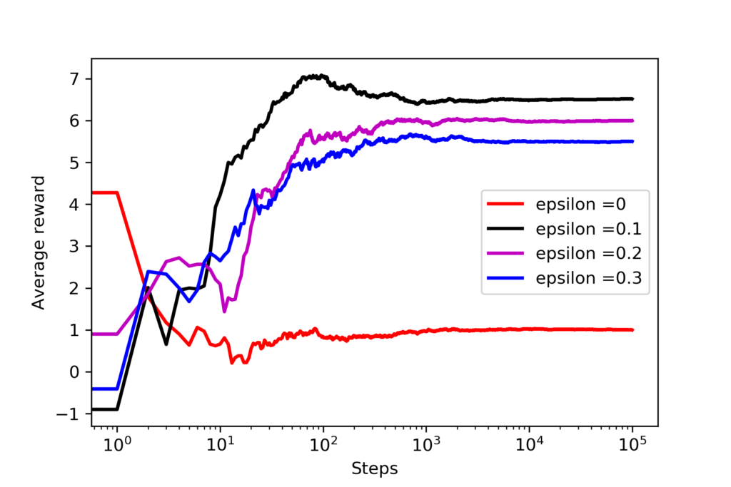
Figure 2: Simulation of the epsilon-greedy action value approach for solving the multi-armed bandit problem.

Here, it should be emphasized that we have tested the solution approach by only drawing a single realization of action values (code line 16). This is done for brevity in the post. In a more detailed analysis, we need to draw true action values (code line 16) from some random distribution and run the approach many times, and then we need to average the results, to get a better insight into the algorithm performance. However, we can still observe from figure 1 that even for a single realization of true action values, the performance of the algorithm highly depends on the selection of the epsilon value. The pure greedy approach (red line) does not produce the best results. The average reward converges to $1$ and that is one of the true action values that are entries of the vector of true action values defined on the code line 16. On the other hand, we can observe that for epsilon=0.1, we obtain the best results. The average reward approaches to $6.5$ , and that is very close to $7$ which is one of the true action values for the action $5$ . In fact, action $5$ should produce the best performance since it has the highest action value. We can see that the algorithm is able to find the most appropriate action value. We can also track how many times a particular action is being selected by inspecting “howManyTimesParticularArmIsSelected “, for epsilon=0.1, we obtain

Bandit2.howManyTimesParticularArmIsSelected
Out[40]: array([ 1443.,  1433.,  1349.,  1387., 91501.,  1499.,  1388.])

Clearly, the action number $5$ is selected most of the times, so we are very close to the optimal performance!

Some form of cross-validation or grid search can be used to find the most optimal value of the epsilon parameter. Of course, there are many other approaches for solving the multi-arm bandit problem. However, since this is an introductory tutorial, we do not cover all the approaches.

That would be all. I hope that you have found this tutorial useful. If you did please consider supporting this tutorial webpage.

Motivational Examples

Solution of the Multi-Armed Bandit Problem

Python Code that Simulates Multi-Armed Bandit Problem and Epsilon-Greedy Action Value Method

admin

You might also like

Solve Ordinary Differential Equations in Python by Using odeint() Function

Clear Graphical and Mathematical Explanation of Yaw, Pitch and Roll Euler Angles – Part 2

Correct and Clear Explanation of Linearization of Dynamical Systems