Introduction to root locus method with example and MATLAB code – Part 1 – Fusion of Engineering, Control, Coding, Machine Learning, and Science

In this post, we introduce the root locus technique. This technique is used to quickly sketch the locations of the closed loop poles when a parameter of the feedback system is varied. We explain a procedure for sketching a root locus graph.

Among other benefits, the root locus graph is very useful for selecting the control parameter(s) that will ensure

– That the closed-loop system is stable.
– That the closed loop system response has a prescribed damping ratio and natural frequency.

The closed-loop system is shown in Fig. 1 below.

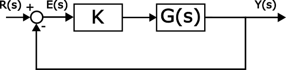
In Fig. 1, $R(s)$ is the reference signal in the Laplace domain, $E(s)=R(s)-Y(s)$ is the error in the Laplace domain, $Y(s)$ is the output in the Laplace domain, $G(s)$ is the transfer function of the plant, and $K\in \mathbb{R}$ is a control parameter that we want to design such that the closed loop system is stable and such that predefined tracking performance is satisfied. We assume that the transfer function $G(s)$ can be represented as follows

(1) $\begin{align*}G(s)=\frac{b(s)}{a(s)}\end{align*}$

where $b(s)$ is a polynomial of degree $m$ and $a(s)$ is a polynomial of degree $n$ . We assume that $m\le n$ (this is a standard assumption that is often met in practice).

Obviously, the closed-loop transfer function is given by the following equation

(2) $\begin{align*}W(s)=\frac{KG(s)}{1+KG(s)}\end{align*}$

The poles of the closed-loop system, are determined as the roots of the following equation

(3) $\begin{align*}1+KG(s)=0\end{align*}$

Obviously, as the parameter $K$ is varied the poles of the system will vary. The root locus of the system can be defined as follows.

The root locus is the set of values of $s$ for which (3) is satisfied as $K$ goes from $0$ to $\infty$ .

So, technically speaking, to construct the root locus, we vary the parameter $K$ , and for every value of $K$ we compute the poles and plot them in the s complex plane. However, this is a tedious job, since we have an infinite number of poles. Luckily, there are several guidelines that can help us to approximately sketch the root locus by hand. In the sequel, we explain these guidelines by using an example.

First, we explain how to sketch the root locus graph by hand, and then we explain how to use MATLAB to accurately draw the root locus graph.

We consider the following example

(4) $\begin{align*}G(s)=\frac{s+1}{s^2}\end{align*}$

This is an open-loop transfer function of a plant. The open-loop poles are

(5) $\begin{align*}p_{1}=0,\;\; p_{2}=0\end{align*}$

and the zero is

(6) $\begin{align*}z_{1}=-1\end{align*}$

We have $n=2$ poles and $m=1$ zeros.

In the sequel, we describe the steps for approximately constructing the root locus graph.

STEP 1:

Mark poles and zeros on the graph.
Denote the starting points. The starting points of the root locus graph are obtained for $K=0$ . These points are actually poles of the transfer function G(s) (open-loop transfer function).
Denote the “obvious” end points of the root locus graph. Some of the end points are the zeros of G(s), and the remaining $n-m$ points are at points at infinity (asymptotes of these infinity directions will be determined later).

admin

You might also like

Dynamical Model of a Tank (Reservoir) Filled with Liquid and Simulation in Python

Pole Placement Example 1- Design PID Controller to Achieve Desired Closed-Loop Behavior

Arduino Motor Connections and Arduino Code for the Differential Drive Robot – Tutorial 3