Feedback Linearization and Control of the Fluid Level in a Tank (Reservoir) – Simulink and MATLAB Implementation. – Fusion of Engineering, Control, Coding, Machine Learning, and Science

In this control engineering, process control, and control theory tutorial, we explain how to use feedback linearization to design a controller for controlling the fluid level in a tank or a reservoir. We will come up with a very elegant control algorithm that does not rely upon classical linearization that depends on computing the partial derivatives. Instead, we will design a control algorithm that will cancel the nonlinearities in the system. After the nonlinearities are canceled, we can use the classical linear control theory to design a controller. In fact, the controller will be nonlinear, however, the closed-loop system will become linear. This relatively simple but effective idea can be generalized to systems of tanks connected with each other and to several tanks controlled by several pumps. The feedback linearization approach has a number of advantages over the classical PID control. The most important advantage of this control algorithm is that it is global and it can guarantee asymptotic stability across a very large range of states and control inputs. On the other hand, the PID controller with fixed parameters usually does not perform well over a large range of states and control actions. It has to be tuned for specific and narrow ranges of states and control actions. However, the main disadvantage of feedback linearization is that it requires precise knowledge of the model parameters.

In this control tutorial, we also explain how to implement and simulate a feedback linearization controller for fluid level control in Simulink and MATLAB.

The YouTube tutorial accompanying this webpage is given below.

Problem Description and Feedback Linearization

We consider a tank filled with an incompressible fluid shown below.

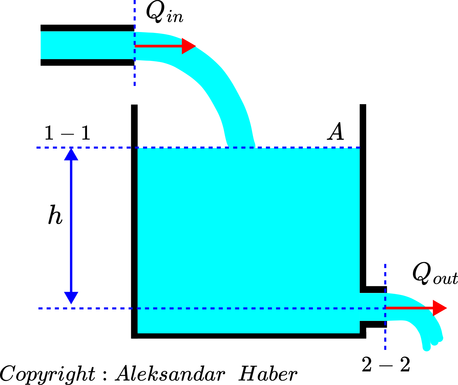
We consider a tank with a cross-section area of A filled with an incompressible fluid. The fluid level at the time instant $t$ is $h$ . The input (volumetric) flow rate to the tank is denoted by $Q_{in}$ . The output (volumetric) flow rate of the tank is denoted by $Q_{out}$ . We assume that the output flow is passive (not actively controlled). We assume that the cross-section of the hole is much smaller than the cross-section A of the tank. We assume that we can control the input flow rate $Q_{in}$ . This input flow rate is created and delivered by a pump.

Our control objective is to control the fluid level $h$ . Let the desired fluid level be denoted by $h_{des}$ . This is the set point for our control algorithm. The goal of the control algorithm is to make the actual fluid level $h$ to be as close as possible to the desired fluid level $h_{des}$ . We assume that the fluid level $h$ can be measured by using the fluid level sensor.

In our previous tutorial given here, we derived a nonlinear model of the fluid level inside of the tank. The nonlinear differential equation is given by

(1) $\begin{align*}\frac{\text{d}h}{\text{d}t}=\frac{1}{A}\cdot Q_{in}-\frac{c}{A}\cdot \sqrt{h}\end{align*}$

where $c$ is a constant that depends on the discharge constant and the gravitational acceleration constant.

The first step in deriving the feedback linearization algorithm is to define the control error. The control error is defined by the following equation

(2) $\begin{align*}e=h_{des}-h\end{align*}$

The goal of the control algorithm is to drive the control error $e$ as close as possible to zero. The control input that cancels the nonlinearity in (1) is defined as follows

(3) $\begin{align*}Q_{in}=c\sqrt{h}+pe\end{align*}$

where $p$ is a control parameter that is selected by the user. By substituting (3) in (1), we obtain

(4) $\begin{align*}\frac{\text{d}h}{\text{d}t} & =\frac{1}{A}\big(c\sqrt{h}+pe \big)-\frac{c}{A} \sqrt{h} \\\frac{\text{d}h}{\text{d}t} & =\frac{c}{A} \sqrt{h}+\frac{p}{A}e -\frac{c}{A}\sqrt{h} \\\end{align*}$

And finally, we obtain

(5) $\begin{align*}\frac{\text{d}h}{\text{d}t} & =\frac{p}{A}e \end{align*}$

Next, we take the first derivative of the error equation (2)

(6) $\begin{align*}\dot{e}=\dot{h}_{des}-\dot{h}\end{align*}$

Since $h_{des}$ is constant, we have that $\dot{h}_{des}=0$ . Consequently, from (6), we have

(7) $\begin{align*}\dot{e}=-\dot{h}\end{align*}$

By substituting (5) in (7), we obtain

(8) $\begin{align*}\dot{e} & =-\frac{p}{A}e \end{align*}$

This equation represents the error dynamics. The last equation represents the closed loop dynamics. It should be observed that the closed-loop dynamics does not depend on the nonlinear terms. That is, the closed-loop dynamics is completely linearized despite the fact that the original system is nonlinear. The control algorithm (3) cancels the model nonlinearities. Also, it should be observed that the control algorithm is nonlinear, and the closed-loop system is linear!

From the equation (8), we can observe that for any positive value of $p$ , the closed-loop system is asymptotically stable.

By increasing the parameter $p$ we can have a faster convergence of the control error (faster response of the closed loop system). However, from (3) we can see that the larger values of $p$ produces a larger value of the control input. Due to the actuator saturation, this is not desirable. There should be a trade-off between the speed of convergence (response) and how large is the control input.

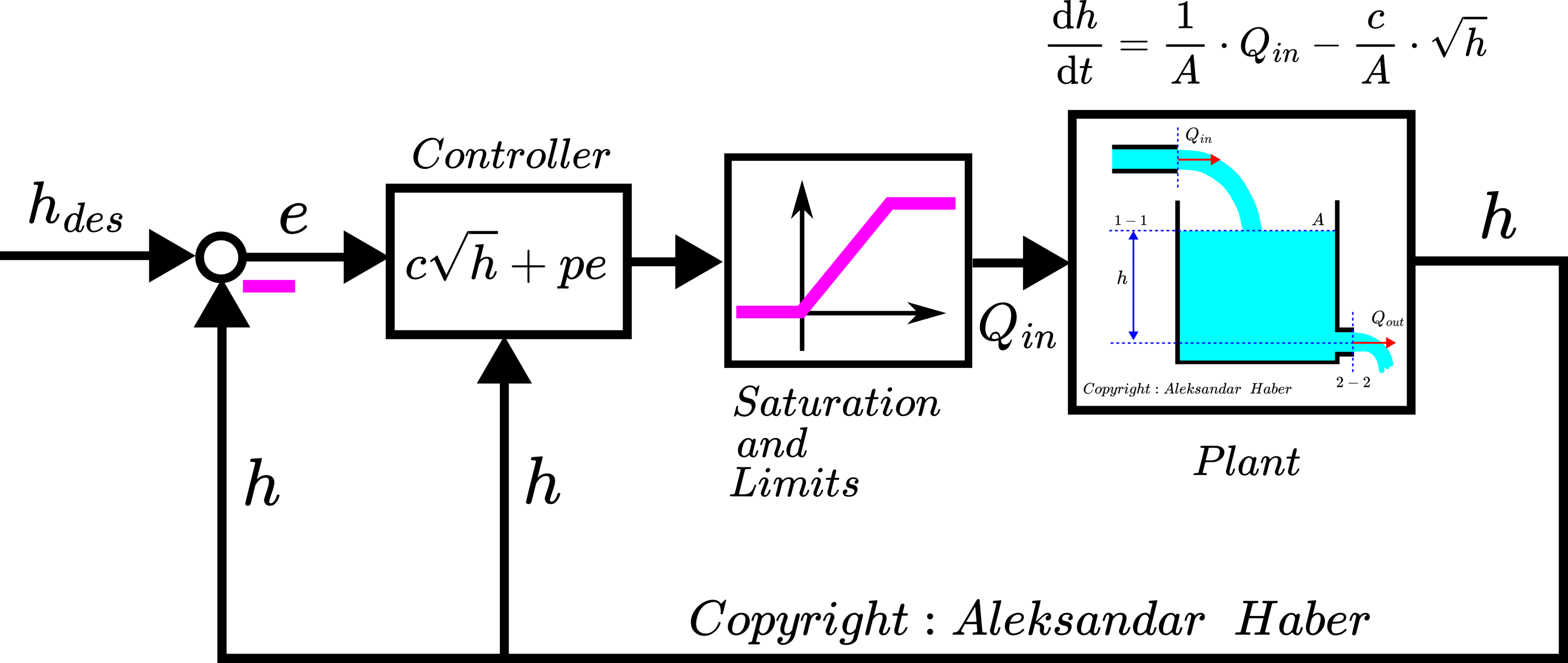
The block diagram of the feedback control system is shown below. This block diagram helps us to implement the control algorithms in Simulink and MATLAB. In this block diagram, we added a saturation and limit block. This block models the fact that a pump cannot produce a negative flow rate and that a pump cannot produce an infinite flow rate. That is, the flow rate is between 0 and some maximum value of the flow rate that the pump can physically deliver.

Problem Description and Feedback Linearization

admin

You might also like

Policy Iteration Algorithm in Python and Tests with Frozen Lake OpenAI Gym Environment- Reinforcement Learning Tutorial

Python Control Systems Library Tutorial 2: Define State-Space Models, Generate Step Response, Discretize, and Perform Basics Operations

Solve Optimization Problems in C/C++ by Using NLopt Library