Nonlinear Model Predictive Control – MPC – Tutorial 1: Basic Formulation and Solution in MATLAB – Fusion of Engineering, Control, Coding, Machine Learning, and Science

In this tutorial series, we explain how to formulate and numerically solve different versions of the nonlinear Model Predictive Control (MPC) problem. We implement the solution in MATLAB. The focus of this series is mainly on the practical implementation without going too deep into the theoretical aspects of nonlinear MPC.

You are currently reading Tutorial 1. In this tutorial, we explain how to formulate an open-loop nonlinear MPC problem and how to approximate its solution in MATLAB.

Before reading this tutorial and watching the video, we suggest that you go over our previous tutorial on the linear MPC implementation given here.

The developed MATLAB code can be found over here (fee needs to be paid). The YouTube tutorial explaining the implementation is given below.

Disclaimer: The algorithm, MATLAB implementation, and the main ideas presented on this webpage and in the accompanying video are an intellectual and digital ownership of the author: Aleksandar Haber. This tutorial should not be reproduced or reposted on other websites. This tutorial should NOT be used as a part of the official curriculum and course provided by universities or educational institutions or companies without the written consent of the author. The developed algorithm and codes should NOT be used in commercial applications and should NOT be used for academic research without the written consent of the author.

For some applications, it is also possible to use the code after paying an appropriate fee. Any unlawful or unauthorized use might induce legal lawsuits.

To cite this tutorial and all other tutorials, cite this report that is in preparation:

“Practical Introduction to Nonlinear Model Predictive Control with MATLAB Implementation”. Technical Report, Number 1, A. Haber, 2024.

Continuous-time Formulation of the Open-Loop Nonlinear Model Predictive Control Problem

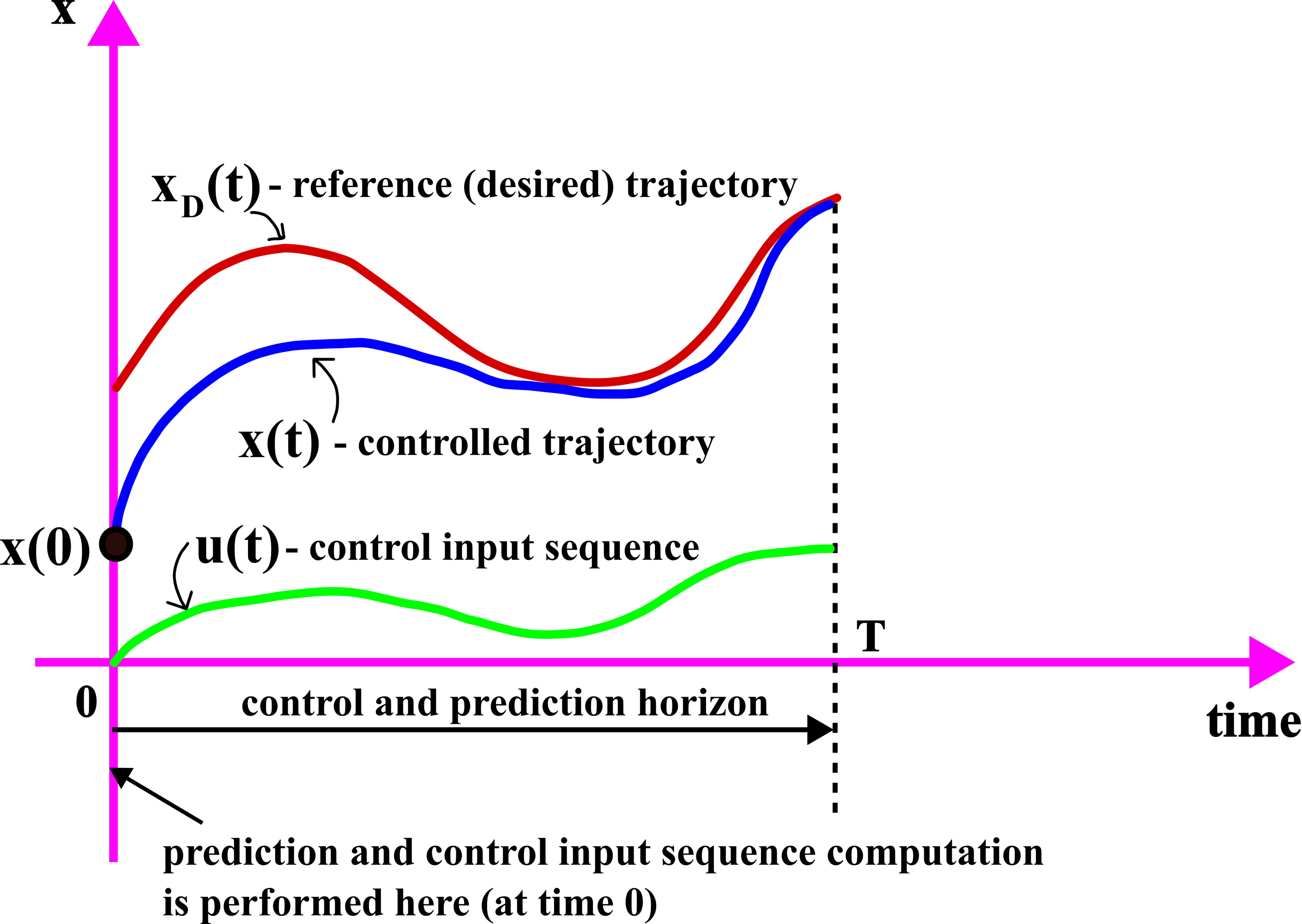
Here, for presentation clarity and completeness, we first briefly formulate a continuous-time open-loop MPC problem. We focus on the open-loop control problem. The open-loop means that we predict and compute the complete future control input sequence at the initial time step, without shifting the time step and without observing the state at the shifted time step. That is, we assume that once it is computed at the initial time step, the complete future control sequence is applied at the subsequent time steps. This strategy can easily be modified to develop a closed-loop MPC algorithm (see our previous tutorial given here).

Here it should be kept in mind that the continuous-time formulation is rarely used in practice. The issue is that this problem is infinite-dimensional, and usually, it cannot be solved directly. Instead, this problem is usually discretized, and additional assumptions are introduced before it can be solved. This will be explained in the next section.

We consider a nonlinear dynamical system in the general form (we will introduce examples later on):

(1) $\begin{align*}\dot{\mathbf{x}}=\mathbf{f}(\mathbf{x},\mathbf{u})\end{align*}$

where

$\mathbf{x} = \mathbf{x}(t) \in \mathbb{R}^{n}$ is the n-dimensional state vector.
$\mathbf{u} = \mathbf{u}(t) \in \mathbb{R}^{m}$ is the m-dimensional control input vector.
$\mathbf{f}$ is a nonlinear state function that maps states and inputs into the n-dimensional derivative vector of states.

The goal of the MPC algorithm is to track a reference (desired) state trajectory. This trajectory should be designed by the user. In typical position control of mechanical systems, this trajectory consists of the user-defined position and velocity profiles. Let the desired reference trajectory be denoted by $\mathbf{x}_{D}(t) \in \mathbb{R}^{n}$ .

Before we formulate the nonlinear MPC problem, we need to introduce the concept of the continuous-time prediction and control horizon denoted by $T$ . The continuous-time prediction and control horizon $T$ denotes the time duration of the time horizon over which we predict the state trajectory as well as formulate and solve the control problem. The prediction and computation are performed at the initial time step (time step 0) of the prediction and control horizon, and the computed control sequence is applied to the actual system during the control horizon.

We assume that the complete state vector at the beginning of the prediction and control horizon is given or directly measured. In the MPC problem formulation given below, we assume that the start time instant of the prediction and control horizon is $0$ . Consequently, we assume that $\mathbf{x}(0)$ is given. The MPC problem is illustrated in Fig. 1 below.

The nonlinear MPC problem for tracking a reference trajectory $\mathbf{x}_{D}(t)$ can be defined as follows.

(2) $\begin{align*}& \min_{u(t)} \int_{0}^{T} \big( \mathbf{x}_{D}(t) - \mathbf{x}(t))^{T} Q(t) \big( \mathbf{x}_{D}(t) - \mathbf{x}(t)) \text{d}t \\& \text{subject to: } \\& \dot{\mathbf{x}}=\mathbf{f}(\mathbf{x},\mathbf{u}) \\& \mathbf{u}_{\text{min}} \le \mathbf{u}(t) \le \mathbf{u}_{\text{max}},\;\; 0 \le t \le T\end{align*}$

In (2),

$Q(t) \in\mathbb{R}^{n}$ is the weighting matrix penalizing the state. We can use this matrix to tune the MPC control algorithm.
$\mathbf{u}_{\text{min}}$ and $\mathbf{u}_{\text{max}}$ are the constant and known vectors defining the control input bounds. They encode the physical limitations of the actuators.

Note that the cost function in (2) is an integral over time of the weighted control error (the term $\mathbf{x}_{D}(t) - \mathbf{x}(t)$ is the control error). Also, in this tutorial, for simplicity and brevity, we have only penalize the control inputs and not state trajectories. State constraints can also easily be incorporated into the optimization problem. This will be explained in our future tutorials.

If we would be able to somehow solve the optimization problem (2), then the solution would be a continuous-time control input function

(3) $\begin{align*}\hat{\mathbf{u}}(t,\mathbf{x}(0))\end{align*}$

However, in the most general case, it is practically impossible to compute an analytical form of the control input function given by (3). One of the main difficulties is that the optimization (2) is infinite-dimensional.

The way to solve this problem is to approximate the problem by a finite-dimensional problem. This is explained in the next section.

Discrete-time and Discretized Formulation of the Open-Loop Nonlinear Model Predictive Control Problem

The first step is to introduce a finite-dimensional control input sequence. We assume that instead of searching for a continuous time control input sequence (3), we search for a discrete-time and finite control input sequence

(4) $\begin{align*}\mathbf{u}_{0},\;\; \mathbf{u}_{1}, \;\; \mathbf{u}_{2},\;\; \ldots, \;\; \mathbf{u}_{N-1}\end{align*}$

where

(5) $\begin{align*}\mathbf{u}_{k}=\mathbf{u}(t=kh),\;\; k=0,1,2,3,\ldots, N-1\end{align*}$

and where $h>0$ is a discretization constant, and $k$ is a discrete-time instant. Here, the last time instant $t=(N-1)h$ corresponds to the control horizon $T$ . That is, $t=T=(N-1)h$ . In this way, we split the prediction and control time horizon $[0,T]$ into the $N$ equidistant time instants:

(6) $\begin{align*}t=0, h, 2h, 3h, \ldots, (N-1)h=T\end{align*}$

The positive integer number $N$ is called the discrete-time prediction and control horizon.

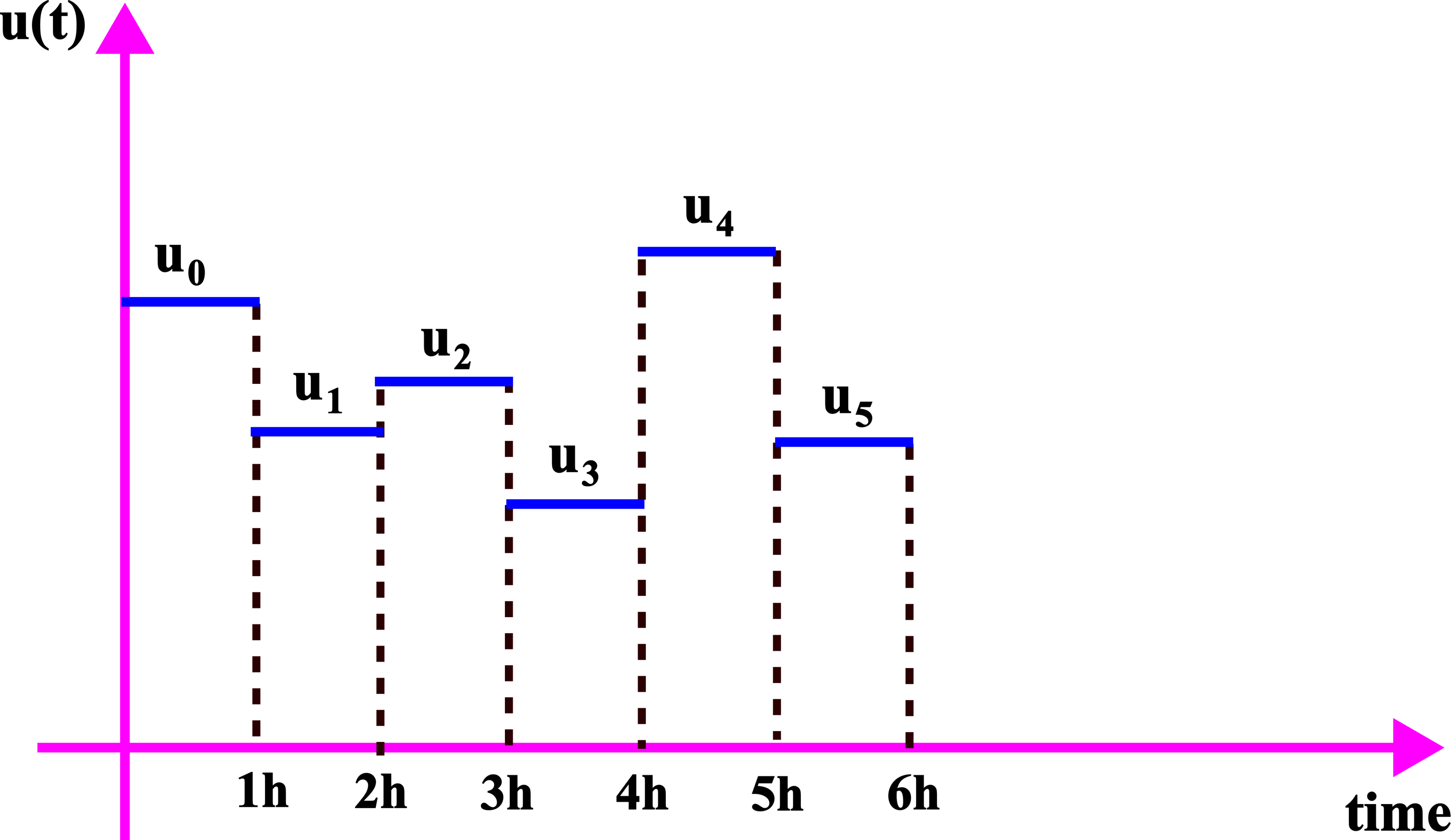
Next, we assume that the control inputs are constant between the discrete-time instants $k\cdot h$ and $(k+1)\cdot h$ . That is, we assume the following

(7) $\begin{align*}u(t)=u_{k}=\text{const},\;\; \forall t\in [kh,(k+1)h), \;\; k=0,1,2,\ldots, N-1 \end{align*}$

The control inputs are shown in the figure below.

The next step is to discretize the continuous dynamics (1). Here, we can use explicit or implicit discretization schemes or even the discretization scheme used by MATLAB’s ode45() solver (we actually use the ode45 solver in our MATLAB simulations). For the presentation clarity, we will formally use the discretized dynamics obtained by using an explicit time-forward discretization. By discretizing (1) and under the assumption of the constant input between the time samples, we obtain the discrete-time state equation representing the discretized dynamics:

(8) $\begin{align*}\mathbf{x}_{k+1}=\mathbf{g}(\mathbf{x}_{k},\mathbf{u}_{k})\end{align*}$

where $\mathbf{g}(\cdot)$ is the discretized state-space dynamics, and $\mathbf{x}_{k}$ is the discretized state vector at the time instant $t=k\cdot h$ . That is, $\mathbf{x}_{k}=\mathbf{x}(t=k\cdot h)$ .

Note that the equation (8) is written only for presentation clarity and in order to illustrate the main ideas. In the MATLAB implementation, we will not use this equation, instead, we will use the ode45 solver to obtain a discrete-time state sequence $\mathbf{x}_{k}$ .

Next, we discretize the cost function (2). By approximating the integral by a sum, we obtain the following cost function

(9) $\begin{align*}\min_{\mathbf{u}_{0},\mathbf{u}_{1},\mathbf{u}_{2},\ldots, \mathbf{u}_{N-1} } \sum_{i=1}^{N} h \cdot \big( \mathbf{x}_{D,i} - \mathbf{x}_{i})^{T} Q_{i} \big( \mathbf{x}_{D,i} - \mathbf{x}_{i}) \end{align*}$

In (9):

$\mathbf{x}_{D,i}$ is the discretized reference (desired) trajectory at the time instant $t= i\cdot h$ . That is, $\mathbf{x}_{D,i}=\mathbf{x}_{D}(t=ih)$ .
$Q_{i}$ is the weight function at the time instant $t= i\cdot h$ . That is, $Q_{i}=Q(t=ih)$ .

Finally, we obtain the discrete-time formulation of the nonlinear model predictive control (MPC) problem

(10) $\begin{align*}&\min_{\mathbf{u}_{0},\mathbf{u}_{1},\mathbf{u}_{2},\ldots, \mathbf{u}_{N-1} } \sum_{i=1}^{N} h \cdot \big( \mathbf{x}_{D,i} - \mathbf{x}_{i})^{T} Q_{i} \big( \mathbf{x}_{D,i} - \mathbf{x}_{i}) \\& \text{subject to: } \\& \mathbf{x}_{i+1}=\mathbf{g}(\mathbf{x}_{i},\mathbf{u}_{i}),\;\; 0 \le i \le N-1 \\& \mathbf{u}_{\text{min}} \le \mathbf{u}_{i} \le \mathbf{u}_{\text{max}},\;\; 0 \le i \le N-1\end{align*}$

Let us group all the optimization variables in a single vector

(11) $\begin{align*}\bar{\mathbf{u}}=\begin{bmatrix}\mathbf{u}_{0} \\ \mathbf{u}_{1} \\ \vdots \\ \mathbf{u}_{N-1} \end{bmatrix}\end{align*}$

When implementing the solution of the optimization problem (10), it is important to keep in mind the following

Any optimization solver for the above problem iteratively computes the optimization variable $\bar{\mathbf{u}}$ , starting from some guess of $\bar{\mathbf{u}}$ . When $\bar{\mathbf{u}}$ is fixed, and due to the fact that the initial condition $\mathbf{x}_{0}$ is known, we can simulate the discretized dynamics (8) to obtain the state sequence $\mathbf{x}_{1}, \mathbf{x}_{2},\ldots, \mathbf{x}_{N}$ . That is, in every iteration of the optimization solver, the discrete states in the cost function can be substituted by their numerical values. Since the reference trajectory is known, in every iteration of the optimization solver, we can evaluate the cost function. This is enough for implementing the solution of the optimization problem in MATLAB. We can use an interior point method to solve the problem.
We do not need to know the gradients of the cost function in order to implement the solution in MATLAB. This is explained in the video. However, by computing the gradient, we can significantly speed up the computations. This will be explored in our future tutorials.

Examples

We will test the MPC algorithm by using two examples. The first example is a linear mass-spring-damper system in the state-space form

(12) $\begin{align*}& \dot{x}_{1}=x_{2} \\& \dot{x}_{2} = -\frac{c}{m}x_{1}-\frac{d}{m}x_{2}+\frac{1}{m}u\end{align*}$

where $c$ , $d$ , and $m$ are the model constants.

The second example is a nonlinear system represented by the following state-space model

(13) $\begin{align*}& \dot{x}_{1}=x_{2} \\& \dot{x}_{2} = 2gx_{1}e^{-gx_{1}^{2}}\Big(bx_{1}^{2}+cx_{1}^{3}+dx_{1}^{4} \Big) \\& -e^{-gx_{1}^{2}}\Big(2bx_{1}+3cx_{1}^{2}+4dx_{1}^{3} \Big)-nx_{2}+u \end{align*}$

Control Results – First Example

The first example is defined by the following parameters: $m=1$ , $c=1$ , and $d=1$ .

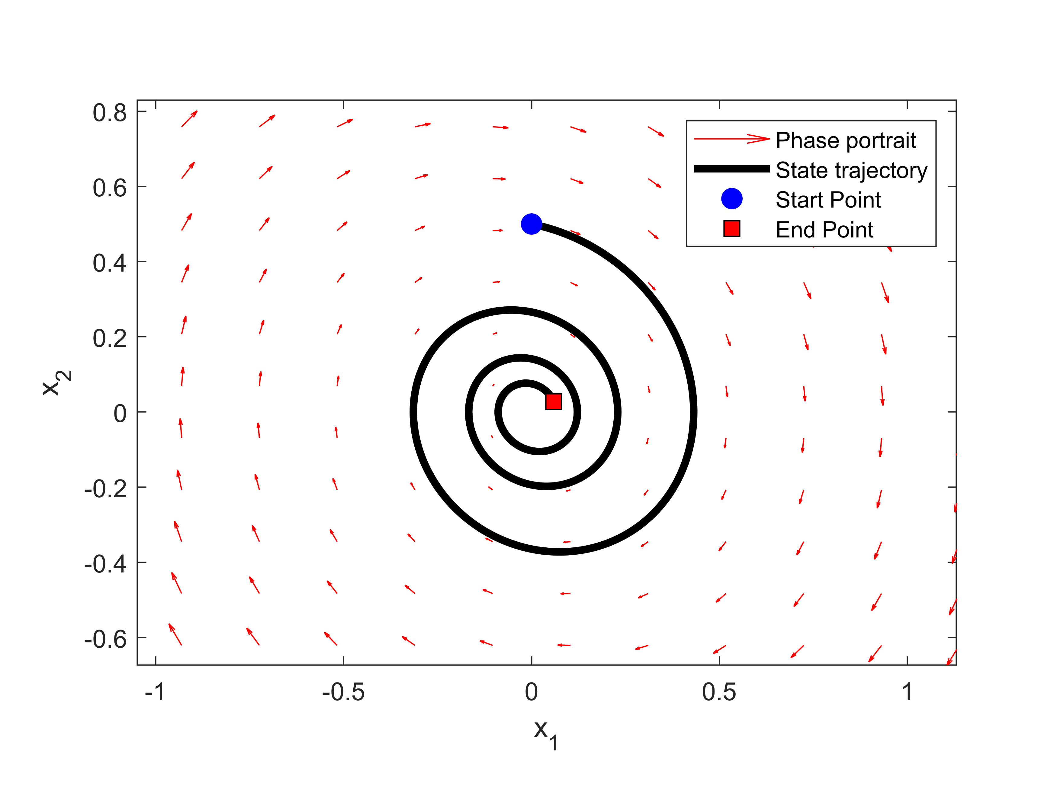
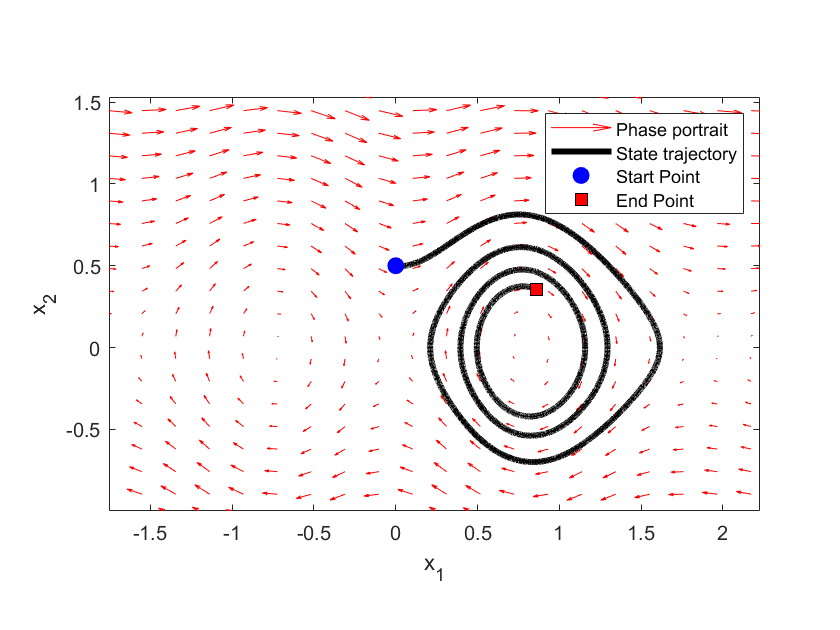
The figure below shows a simulated phase portrait and a single trajectory.

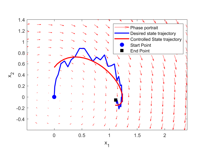
Fig.3: Phase portrait and a single trajectory of the first example.

The figure below shows the desired and controlled state-space trajectory. The controlled trajectory is controlled by using the solution of the MPC problem.

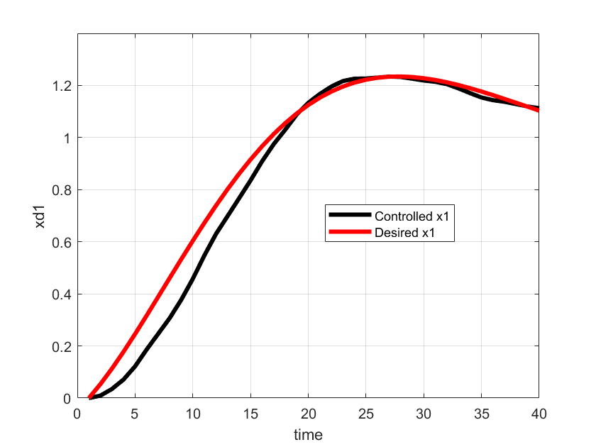
Fig. 4: Desired and controlled state-space trajectory.

The time representation of the desired value of $x_{1}$ and the controlled value of $x_{1}$ is shown below.

Fig. 5: Desired and controlled $x_{1}$ .

Control Results – Second Example

The second example is defined by the following parameters: $g=1$ , $b=-1$ , $c=-0.1$ , $d=0.5$ , and $n=0.1$ .

The phase portrait is given below and a single trajectory is given in the figure below.

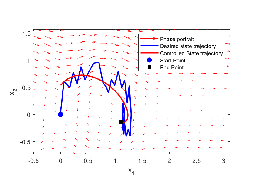
Fig.6: Phase portrait and a single trajectory of the first example.

The figure below shows the desired and controlled state-space trajectory. The controlled trajectory is controlled by using the solution of the MPC problem.

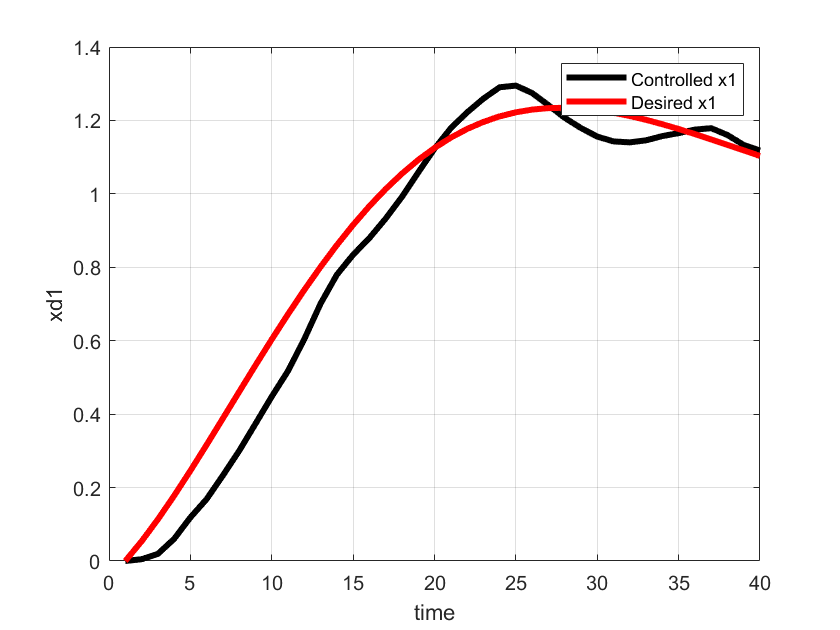
Fig. 7: Desired and controlled state-space trajectory.

The time representation of the desired value of $x_{1}$ and the controlled value of $x_{1}$ is shown below.

Continuous-time Formulation of the Open-Loop Nonlinear Model Predictive Control Problem

Discrete-time and Discretized Formulation of the Open-Loop Nonlinear Model Predictive Control Problem

Examples

Control Results – First Example

Control Results – Second Example

admin

You might also like

Control Systems Lecture: Overshoot and Peak Time as Functions of Damping Ratio and Natural Undamped Frequency – Complete Derivation

Exercises for ENS 100 – Introduction to Engineering

Optional Homework Assignment: Solving beam differential equation in the reversed coordinate system