10. Decomposition of Time-Series in Python: Trend and Seasonal (Periodic) Components – Fusion of Engineering, Control, Coding, Machine Learning, and Science

In this post, we explain how to decompose a time series into trend and seasonal (periodic) components. The decomposition step is necessary in order to remove deterministic components of a time series and in order to make the time series to be as close as possible to a statistically stationary signal. We use the Python Statsmodels library to perform decomposition. A YouTube video accompanying this post is given below.

Briefly speaking, a time series $x_{k}$ , where $k$ denotes a discrete-time index, can be decomposed as follows

(1) $\begin{align*}x_{k}=a_{k}+b_{k}+r_{k}\end{align*}$

where $a_{k}$ is a trend component, $b_{k}$ is a seasonal (periodic) component, and $r_{k}$ is a residual component that is often a stochastic time series signal.

In the sequel, we present a Python code that demonstrates how to peform time-series decomposition. We construct an artificial time series that is a discrete-time version of a continuous-time domain function having the following form

(2) $\begin{align*} x(t) = \underbrace{k_{0}sin(\omega t)}_{\text{periodic component - seasonality}}+\underbrace{k_{1}+k_{2}t+k_{3}t^{2}}_{\text{trend component}} \end{align*}$

where $\omega = 2\pi / T$ , where $T$ is a period, $k_{0},k_{1},k_{2},$ and $k_{3}$ are constants, and $t$ is time.

In the sequel, we present the code for decomposing time-series signals. To perform the decomposition, we use the Statsmodels Python Library. The following code lines are used to import the necessary libraries and to define time series.

# -*- coding: utf-8 -*-
"""
Decomposition of time series into trend and seasonality components

Author:
    
    Aleksandar Haber
    March 2021

"""
import matplotlib.pyplot as plt
import numpy as np
from statsmodels.tsa.seasonal import seasonal_decompose

total_duration=100
step=0.01

time=np.arange(0,total_duration, step)

# period of the sinusoidal signal in seconds
T= 15

# period component
series_periodic = np.sin((2*np.pi/T)*time)

#add a trend component
k0=2
k1=2
k2=0.05
k3=0.001

series_periodic=k0*series_periodic
series_trend=k1*np.ones(len(time))+k2*time+k3*time**2
series=series_periodic+series_trend

We use the Statsmoldes function “seasonal_decompose” to perform the decomposition. As an input parameter of this function, we need to specify the period of time series. In the continuous-time domain, the period of the sinusoidal signal is $T=10$ seconds. However, the period parameter for the “seasonal_decompose” function is equal to the length of this period in the discrete-time domain. In code line 16 we have defined a discrete-time step of step=0.01. This implies that the period parameter will be “period=T/step”. In this example, we know the period of the function. However, in many other situations, the period will be uknown. In order to estimate the dominant period, we can compute a power spectral density of the signal, or we can use some other method.

The following code lines perofm the decomposition and generate decomposition graphs.

period = int(T/step)
results = seasonal_decompose(series, model='additive', period=period)
trend_estimate    = results.trend
periodic_estimate = results.seasonal
residual = results.resid

plt.figure(figsize=(12,10))
plt.subplot(411)
plt.plot(series,label='Original time series', color='blue')
plt.legend(loc='best')
plt.subplot(412)
plt.plot(trend_estimate,label='Trend of time series',color='blue')
plt.legend(loc='best')
plt.subplot(413)
plt.plot(periodic_estimate,label='Seasonality of time series',color='blue')
plt.legend(loc='best')
plt.subplot(414)
plt.plot(residual,label='Decomposition residuals of time series',color='blue')
plt.legend(loc='best')
plt.tight_layout()
plt.savefig('decomposition.png')

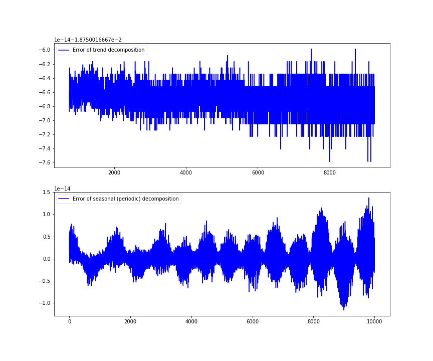
# check the decomposition accuracy of trend and seasonal components

error_trend=series_trend-trend_estimate 
error_periodic=series_periodic-periodic_estimate

plt.figure(figsize=(12,10))
plt.subplot(211)
plt.plot(error_trend,label='Error of trend decomposition', color='blue')
plt.legend(loc='best')
plt.subplot(212)
plt.plot(error_periodic,label='Error of seasonal (periodic) decomposition', color='blue')
plt.legend(loc='best')
plt.savefig('error_trend_periodic.png')

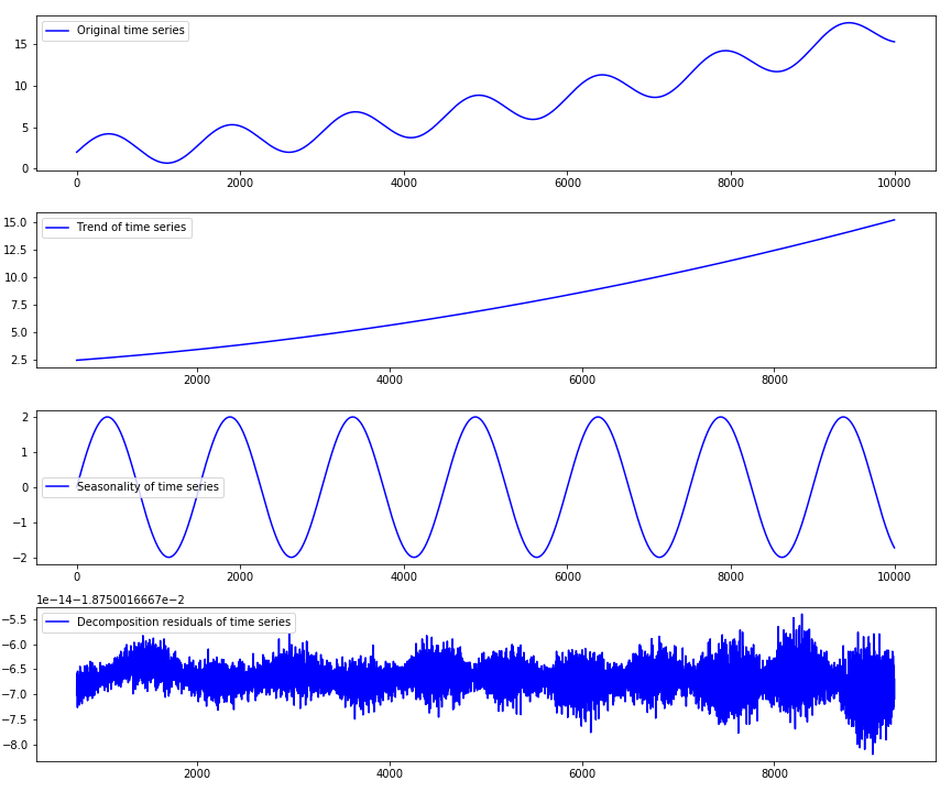
A few comments are in order. Actual decomposition is performed in code line 2. The second input parameter of the function, denoted by “additive”, means that we are performing additive decomposition defined by Eq.(1). Instead of additive decomposition, we can also perform a multiplicative decomposition. The function “seasonal_decompose” returns a structure containing trend, seasonality, and residual components. These components are extracted in code lines 3-5. The original time series and the estimates of trend and seasonal components are shown in Fig. 1. below. This figure also shows the computed residuals.

Figure 1: Decomposition of time-series into trend and seasonality components. Top figure presents the original time series. The second figure from the top is the estimated trend component. The third figure from the top is the estimated seasonality (periodic) components. The bottom figure is the decomposition residual.

The code lines 25-35 are used to compute the errors of seasonal and trend decompositions. We subtract estimated trend and seasonal components from the actual trend and seasonal components that are defined at the beginning of this post. In the end, we plot the computed errors. The errors are shown in Fig. 2. below.

admin

You might also like

Import *.csv and *.txt Numerical Files and Data in MATLAB

Introduction to Kalman Filter: Derivation of the Recursive Least Squares Method

Bonus Homework Assignment – Computation of the Moment of Inertia of an I-beam

Import .csv and .txt Numerical Files and Data in MATLAB