Control Systems Lecture: Open-Loop Control with MATLAB Simulations – Fusion of Engineering, Control, Coding, Machine Learning, and Science

In this post, we introduce an open-loop control approach. We also introduce MATLAB codes that can be used to simulate the dynamics of a system that is controlled using the open-loop control method. A video accompanying this post is given below.

We can use open-loop control when we have perfect knowledge about the system that we want to control, and we do not expect that some unpredictable events or disturbances will affect the system during its operation. Since it does not rely upon feedback information that is collected by sensors, open-loop control is simple and cost-effective.

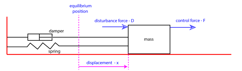
In our previous post, we have explained how to derive a transfer function model of the mass-spring-damper system shown in the figure below. In this post, we explain how to design an open-loop controller for such a system.

The transfer function model has the following form:

(1) $\begin{align*}X(s)=\frac{A}{(\tau_{1}s+1)(\tau_{2}s+1)}F(s)+\frac{B}{(\tau_{1}s+1)(\tau_{2}s+1)}D(s)\end{align*}$

where $X(s),F(s)$ , and $D(s)$ are Laplace transforms of the position $x(t)$ , control force $F(t)$ , and disturbance force $D(t)$ , and $A,B,\tau_{1}$ , and $\tau_{2}$ are constants (for more details see our previous post). For our MATLAB simulations (at the end of this post), we define:

(2) $\begin{align*}W_{1}(s)=\frac{A}{(\tau_{1}s+1)(\tau_{2}s+1)},\;\; W_{2}(s)=\frac{B}{(\tau_{1}s+1)(\tau_{2}s+1)}\end{align*}$

where $W_{1}(s)$ is the transfer function from the control force to the displacement, and $W_{2}(s)$ is the transfer function from the disturbance force to the displacement. A block diagram of the system is shown below.

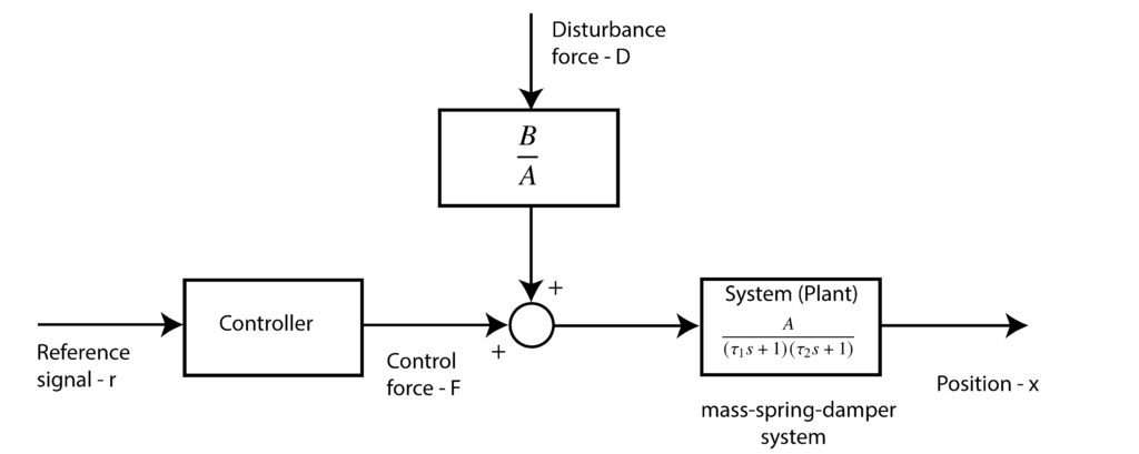
We have deliberately reformulated the system description in order to emphasize different system parts. We have also introduced a controller. The purpose of the controller is to generate the control force $F$ such that the system’s position $x$ (displacement) becomes equal to a reference signal $r$ that represents a desired position of the mass. Our goal is to design such a controller.

For the time being, we are going to exclude the disturbance force, since in practice we often do not have a priori knowledge about disturbances acting on the system. Consequently, the system’s model has the following form

(3) $\begin{align*}X(s)=\frac{A}{(\tau_{1}s+1)(\tau_{2}s+1)}F(s)\end{align*}$

and the controller will have the following form

(4) $\begin{align*}F(t)=Kr(t)\end{align*}$

where $K\in \mathbb{R}$ is an open-loop control gain. Let us assume that the control objective is to keep $r(t)=r_{d}$ , for $t\ge 0$ . Substituting this equation in (4), we obtain

(5) $\begin{align*}F(t)=Kr_{d}\end{align*}$

Applying the Laplace tranform to (5), we obtain

(6) $\begin{align*}F(s)=\frac{K r_{d}}{s}\end{align*}$

Substituting (6) in (3), we obtain

(7) $\begin{align*}X(s)=\frac{A}{(\tau_{1}s+1)(\tau_{2}s+1)}\frac{K r_{d}}{s}\end{align*}$

Next, we recall the final value theorem. The final value theorem states that if all the poles of $s\cdot X(s)$ are in the left half of the s-plane, then

(8) $\begin{align*}\lim_{t \rightarrow \infty} x(t)=\lim_{s \rightarrow 0} sX(s)\end{align*}$

Since in our case, the poles of $s X(s)$ are in the left half of the s-plane (the mass-spring-damper system is asymptotically stable), from (7) and the final value theorem, we obtain

(9) $\begin{align*}x_{ss}=\lim_{t \rightarrow \infty } x(t) = \lim_{s \rightarrow 0}\frac{A K r_{d} }{(\tau_{1}s+1)(\tau_{2}s+1)}\end{align*}$

where $x_{ss}$ is the steady-state position of the mass. From the last equation, we obtain

(10) $\begin{align*}x_{ss}=A \cdot K r_{d}\end{align*}$

Our goal is to make $x_{ss}=r_{d}$ . From (10), we see that this achieved when

(11) $\begin{align*}A\cdot K=1,\;\; K=\frac{1}{A}\end{align*}$

That is, when $K=1/A$ , then $x_{ss}=r_{d}$ . On the other hand, let us see what is the physical meaning of the parameter $A$ . Consider a unit step control force applied to the system

(12) $\begin{align*} F(t)=1\end{align*}$

Then, we have

(13) $\begin{align*}X(s)=\frac{A}{(\tau_{1}s+1)(\tau_{2}s+1)}\frac{1}{s}\end{align*}$

In this case, the steady state system response is computed as follows

(14) $\begin{align*} \tilde{x}_{ss}=\lim_{t\rightarrow \infty} x(t)=\lim_{s\rightarrow 0} sX(s)=\lim_{s\rightarrow 0} \frac{A}{(\tau_{1}s+1)(\tau_{2}s+1)}= A\end{align*}$

That is, the parameter $A$ is the steady-state gain of the open-loop system. Consequently, the open-loop controller gain $K$ should be equal to the inverse of the system open-loop gain. In some sense, the open-loop controller inverts the system. This is also true for more complex open loop dynamic controllers.

Let us now numerically test this control approach.

First, we define the transfer function using the approach explained in this post.

clear, pack, clc
% define system parameters
% mass 
m=10
% damping 
kd=1
% spring constant
ks=100

% control force constant
b=5

% disturbance constant
c=0.1

% Defining transfer functions

% compute the poles
s1=(-(kd/m)+sqrt( (kd/m)^2 -4*(ks/m) ))/2
s2=(-(kd/m)-sqrt( (kd/m)^2 -4*(ks/m) ))/2

tau1= 1/(-s1);
tau2= 1/(-s2);

A=b/ks;
B=c/ks;

s = tf('s');

W1=A/((tau1*s+1)*(tau2*s+1))
W2=B/((tau1*s+1)*(tau2*s+1))

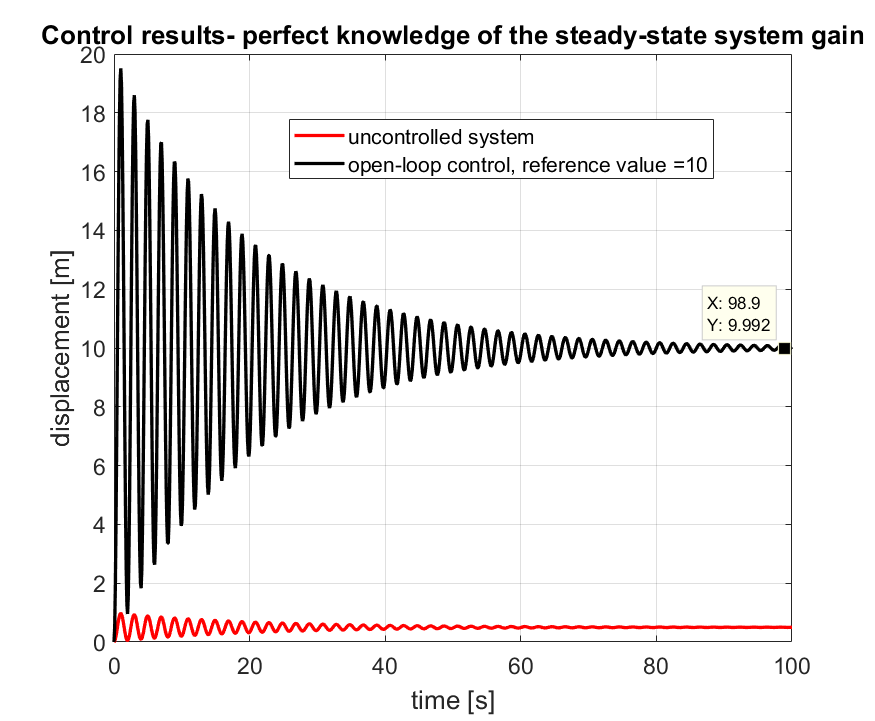
Next, we simulate the system response when the control gain $K$ is computed on the basis of the perfect knowledge of the system steady-state gain $A$ . We assume that the value of the reference signal is 10. That is, the desired mass displacement is 10, and the controller should ensure that the mass reaches this value in the steady-state. The MATLAB code is given below

% this is the response of the system that is not controlled
 desired_position=10;
 time_vector=0:0.1:100;
 input_signal=desired_position*ones(size(time_vector));
 X = lsim(W1,input_signal,time_vector);

 % now, let us add an open loop controller
 K=1/A
 W1_controlled=W1*K
 X_controlled = lsim(W1_controlled,input_signal,time_vector)
 
 
 figure(1)
 % uncontrolled system
 plot(time_vector,X,'r')
 hold on
 % controlled system
 plot(time_vector,X_controlled,'k')

The results are shown in the graph below.

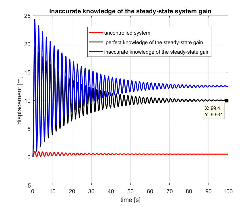
Obviously, there are at least two drawbacks of the open-loop control approach. The first drawback that in practice we often do not know the precise system model. In our case, we might not know accurately, the steady-state system gain. The effect of the lack of precise knowledge of the system gain $A$ on the control system performance is simulated using the code given below.

 %%%%%%%%%%%%%%%%%%%%%%%%%%%%%%%%%%%%%%%%%%%%%%%%%%%%%%%%%%%%%%%%%%%%%%%%%% 
 %            drawbacks of the open loop control approach
 %%%%%%%%%%%%%%%%%%%%%%%%%%%%%%%%%%%%%%%%%%%%%%%%%%%%%%%%%%%%%%%%%%%%%%%%%%
 
 % 1. we do not know the open loop gain A accuratelly
 % for example we assume that the value of A that we know is equal to 0.8*A
 
 K2=1/(0.8*A)
 
 W1_controlled2=W1*K2
 X_controlled2 = lsim(W1_controlled2,input_signal,time_vector)
 
 
 figure(2)
 % uncontrolled system
 plot(time_vector,X,'r')
 hold on
 % controlled system - accurate knowledge of A
 plot(time_vector,X_controlled,'k')
 % controlled system - inaccurate knowledge of A
 plot(time_vector,X_controlled2,'b')

The control results are presented in the graph below.

Also, another drawback of the open-loop control is that the controller completely blind with respect to the disturbance that can act on the system. The disturbances can severely deteriorate the system performance. The code below illustrates the effect of disturbances.

% 2. disturbance is acting on the system
 % compute the response to the disturbance force
 
 time_vector=0:0.1:100;
 disturbance_signal=1000*ones(size(time_vector));
 X_disturbance = lsim(W2,disturbance_signal,time_vector);
 
 % system is linear- so we can do this:
 X_with_disturbance= X_controlled + X_disturbance;
 
 
  figure(3)
 % uncontrolled system
 plot(time_vector,X,'r')
 hold on
 % controlled system - accurate knowledge of A - no disturbance
 plot(time_vector,X_controlled,'k')
 % controlled system - accurate knowledge of A - with disturbance
 plot(time_vector,X_with_disturbance,'b')

The results are shown in figure below.

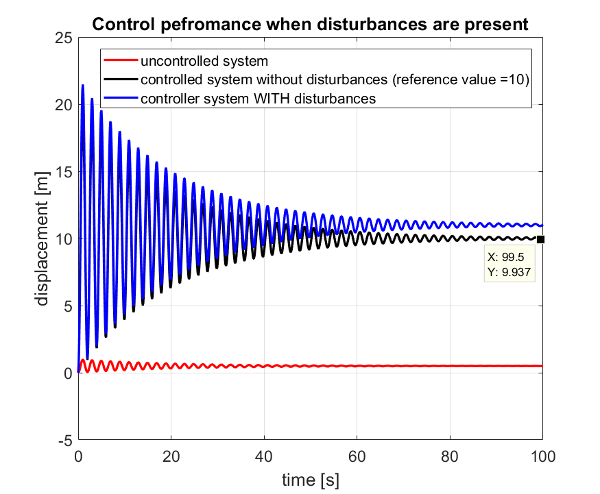
To summarize: open-loop control approach is useful when the system dynamics is known accurately and where there are no unmodeled disturbances acting on the system. The open-loop control approach presented in this post is based on the knowledge of the system steady-state gain. Consequently, we were not able to influence the transient response of the system using this approach. However, there are more advanced open-loop control approaches that can influence the system transient response.

admin

You might also like

Solve Constrained Optimization Problems in Python by Using SciPy Library, minimize() Function and Trust-Region Constrained Method

10. Decomposition of Time-Series in Python: Trend and Seasonal (Periodic) Components

Lambda Functions in Python and Application to Map Function, Filter Function, and Pandas DataFrames