Bode Plots of Integral and Derivative Transfer Functions – Fusion of Engineering, Control, Coding, Machine Learning, and Science

In this control engineering tutorial, you will learn how to quickly sketch (draw) Bode plots of integral and derivative transfer functions. That is, you will learn how to quickly sketch Bode plots of the following transfer functions

(1) $\begin{align*}\frac{1}{s}, \;\; s\end{align*}$

The YouTube video tutorial accompanying this webpage is given below.

The main motivation for learning how to sketch the Bode plots by hand comes from the fact that this knowledge will develop in students the basic intuition of how dynamical systems behave in the frequency domain.

First, we have to introduce a few important concepts. Let $W(s)$ be a transfer function of a linear dynamical system. Then, the sinusoidal transfer function is given by

(2) $\begin{align*}W(j\omega)\end{align*}$

where $j$ is the imaginary unit and $\omega$ is the angular frequency measured in radians per second. That is, the sinusoidal transfer function is obtained by substituting $s$ by $j\omega$ in the transfer function. Next, we can write the sinusoidal transfer function in the polar form

(3) $\begin{align*}W(j\omega)= M(\omega)e^{j\phi(\omega)}\end{align*}$

where

The quantity $M(\omega)$ is called the magnitude or the amplitude ratio of the output sinusoid to the input sinusoid. It is defined by
(4) $\begin{align*}M=| W(j\omega)|=\sqrt{\Big(\text{Re}\big[W(j\omega)\big] \Big)^{2}+\Big(\text{Im}\big[ W(j\omega) \big] \Big)^{2}}\end{align*}$
The quantity $\phi(\omega)$ is called the phase, and it is defined as follows
(5) $\begin{align*}\phi=\tan^{-1} \Big(\frac{\text{Im}\big(W(j\omega)\big) }{\text{Re}\big(W(j\omega)\big) } \Big) \end{align*}$

The phase is expressed either in degrees or in radians.

Next, we need to define the log-magnitude. The log-magnitude is defined as follows:

(6) $\begin{align*}L=20\log_{10}\Big(M\Big)=20\log_{10}\Big( | W(j\omega)|\Big)\;\; \text{expressed in dB}\end{align*}$

Here it should be mentioned that often in graphs log-magnitude $L$ is actually denoted by M(dB), where dB means that the magnitude is actually the log-magnitude.

Now that we have defined the magnitude, log-magnitude, and phase, we can explain the Bode diagram. Essentially, the Bode diagram consists of the following two graphs.

The first graph is the plot of the log magnitude.
The second graph is the plot of the phase.

Both of these graphs are plotted against the angular frequency (or in some cases, just the frequency) on a logarithmic scale.

Bode plot of 1/s

Consider this transfer function

(7) $\begin{align*}W(s)=\frac{1}{s}\end{align*}$

The sinusoidal transfer function is given by

(8) $\begin{align*}W(j\omega)=\frac{1}{j\omega}\end{align*}$

Next, let us obtain the polar form of this transfer function from which we can easily determine the magnitude and phase

(9) $\begin{align*}W(j\omega)=\frac{1}{j\omega}=\frac{1}{j\omega}\cdot \frac{j}{j}=\frac{j}{-\omega}=-\frac{1}{\omega} j \end{align*}$

There are several ways to obtain the polar form of this complex number. We first explain the easiest way. Namely, since

(10) $\begin{align*}-j=e^{-\frac{\pi}{2}j}\end{align*}$

We have

(11) $\begin{align*}W(j\omega)=-\frac{1}{\omega} j=\frac{1}{\omega}e^{-\frac{\pi}{2}j}\end{align*}$

From this expression, we obtain

(12) $\begin{align*}M(\omega)=\frac{1}{\omega},\;\; \phi =-\frac{\pi}{2}\end{align*}$

On the other hand, by applying the defining formula for magnitude and phase to the equation (9), we obtain

(13) $\begin{align*}M=\sqrt{0+\Big( -\frac{1}{\omega}\Big)^{2}}=\frac{1}{\omega}\\\phi =\tan^{-1}\Big(\frac{-\frac{1}{\omega}}{0} \Big)=\tan^{-1}\Big(-\infty \Big)=-\frac{\pi}{2}=-90^{\circ}\end{align*}$

where we should keep in mind that $\omega$ is always positive (there is no need for an absolute value). Consequently, we obtain the log-magnitude

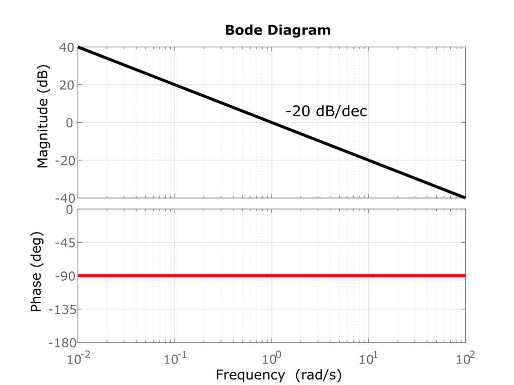
(14) $\begin{align*}L=20\log_{10}\big(M \big)=20\log_{10}\big(\frac{1}{\omega}\big)=-20\log_{10}\big(\omega\big)\end{align*}$

In the Bode plot, this log-magnitude function is a simple line. We obtain the first point on the line by setting $\omega=1$ . From the formula for $L$ , we obtain that for this angular frequency, the value of $L$ is $L(1)=0\; dB$ . Another point can be obtained for $\omega=10$ . We obtain $L(10)=-20\;\; dB$ . We conclude that this line decreases for $20 dB$ for an increase of angular frequency of 10. That is, the slope of this line is $20\;\; dB$ per decade (short notation $20\;\; dB/dec$ ).

The Bode magnitude and phase plot is shown below. Note that the first graph actually shows $L$ . However, we kept $M(dB)$ to be consistent with MATLAB’s way of denoting the log-magnitude. However, the reader of this tutorial should keep in mind that $M(dB)$ is actually $L$ . The Bode diagram (log-magnitude and phase) is shown in the figure below. Note that the frequency on the x-axis is in the logarithmic scale.

Bode plot of the transfer function $1/s$ .

Bode plot of s

We consider the following transfer function

(15) $\begin{align*}W(s)=s\end{align*}$

By using similar steps to the steps used to derive the Bode diagram of the transfer function $1/s$ , we can show that this transfer function has the following magnitude and phase

(16) $\begin{align*}M(\omega)=\omega,\;\; \phi=\frac{\pi}{2}=90^{\circ}\end{align*}$