How To Solve Projectile Motion Problem – Derivation of Kinematic and Dynamics Equations – Fusion of Engineering, Control, Coding, Machine Learning, and Science

In this Physics and AP physics tutorial, we explain how to solve the projectile motion problem. More precisely, in this dynamics and physics tutorial, we treat the problem of projectile motion. We will derive kinematic and dynamics equations describing the trajectory, velocity, and acceleration of a projectile launched with a certain initial velocity. We also derive a formula for the distance that the projectile traveled until it reached the target. The projectile motion analyzed in this video tutorial is important for a number of physical, engineering, and aerospace applications. Consequently, it is very important to thoroughly study this topic and to derive all the equations such that you will know how to apply them in practice.

By practicing this problem you can also prepare yourself for the Advanced Placement (AP) exams: AP Physics 1: Algebra-Based, AP Physics 2: Algebra-Based, AP Physics C: Mechanics, AP Calculus AB – Physics, and Advanced Placement (AP) Calculus. The YouTube lecture accompanying this webpage tutorial is given below.

We solve the following problem: A projectile is launched with the initial velocity $V_{0}$ . The initial velocity is described by the x-projection denoted by $V_{0x}$ and y-projection denoted by $V_{0y}$ . We assume that the air resistance can be neglected. Determine:
a) $x$ and $y$ components of the velocity vector as the function of time.
b) Horizontal and vertical traveled distances as a function of time. That is, determine $x=x(t)$ and $y=y(t)$ .
c) Shape and mathematical function describing the projectile’s trajectory.
d) Horizontal distance that the projectile traveled until it reached the target.

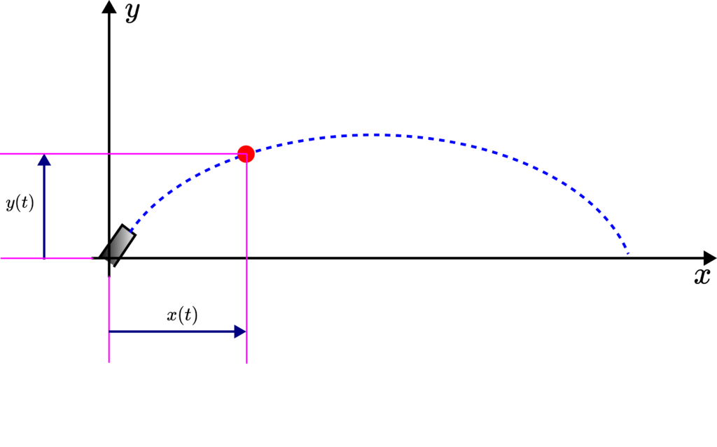
The problem is shown in the figure below.

To solve this problem, we need to start from Newton’s second law. We have

(1) $\begin{align*}m\overrightarrow{a}=m\overrightarrow{g}\end{align*}$

where $m$ is mass, $\overrightarrow{a}$ is the acceleration vector of the projectile, and $\overrightarrow{g}$ is the gravity acceleration. From the last equation, we have

(2) $\begin{align*}\overrightarrow{a}=\overrightarrow{g}\end{align*}$

Next, we introduce the $x(t)$ and $y(t)$ coordinates of the projectile in the figure shown below.

By projecting this equation onto the $x$ equation, we obtain

(3) $\begin{align*}a_{x}=\ddot{x}=0\end{align*}$

where $a_{x}$ is the x projection of the acceleration vector $\overrightarrow{a}$ , and where $\ddot{x}$ is the second derivative of $x(t)$ . The component of the acceleration $a_{x}$ is zero since the gravitational acceleration does not have a projection onto the $x$ axis. From the last equation, we obtain

(4) $\begin{align*}\frac{d\dot{x}}{dt}=0\end{align*}$

By integrating the last equation, we obtain

(5) $\begin{align*}\dot{x}=C_{1}\end{align*}$

where $C_{1}$ is an integration constant. We determine this integration constant from the initial velocity. We have

(6) $\begin{align*}\dot{x}(0)=V_{0x}\end{align*}$

By substituting this initial condition in (5), we obtain $C_{1}=V_{0x}$ . Finally, we obtain

(7) $\begin{align*}\dot{x}=V_{0x}\end{align*}$

This is the solution for the velocity component in the x direction. From the last equation, we obtain

(8) $\begin{align*}\frac{dx}{dt} & =V_{0x} \\dx& =V_{0x}\cdot dt\end{align*}$

By integrating this equation, we obtain

(9) $\begin{align*}x(t)=V_{0x}\cdot t +C_{2}\end{align*}$

We determine the integration constant $C_{2}$ from the initial condition $x(0)=0$ . By substituting this initial condition in (10). We obtain the solution for $x(t)$ :

(10) $\begin{align*}x(t)=V_{0x}\cdot t\end{align*}$

Next, we project the vector (2) onto the $y$ axis. As a result, we obtain

(11) $\begin{align*}a_{y}=\ddot{y}=-g\end{align*}$

where $a_{y}$ is the projection of the acceleration vector $\overrightarrow{a}$ onto the $y$ axis, $\ddot{y}$ is the second derivative of $y(t)$ , and $g$ is the gravity acceleration. From the last equation, we have

(12) $\begin{align*}\frac{d\dot{y}}{dt}=-g\end{align*}$

From the last equation, we have

(13) $\begin{align*}d\dot{y}=-g\cdot dt\end{align*}$

By integrating the last equation, we have

(14) $\begin{align*}\dot{y}=-g\cdot t +C_{3}\end{align*}$

where $C_{3}$ is a constant that needs to be determined from the initial condition. We have

(15) $\begin{align*}\dot{y}(0)=V_{0y}\end{align*}$

By substituting this initial condition in (14), we obtain

(16) $\begin{align*}\dot{y}(0)& =-g\cdot 0 +C_{3} =V_{0y} \\C_{3}&=V_{0y}\end{align*}$

By substituting this initial condition in (14), we obtain

(17) $\begin{align*}\dot{y}=-g\cdot t +V_{0y}\end{align*}$

This is the solution for the velocity component in the y direction. From the last equation, we obtain

(18) $\begin{align*}\frac{dy}{dt}=-g\cdot t +V_{0y}\end{align*}$

From the last equation, we obtain

(19) $\begin{align*}dy=-g\cdot t\cdot dt +V_{0y}\cdot dt\end{align*}$

By integrating the last equation, we obtain

(20) $\begin{align*}y(t)=-g\cdot \frac{t^{2}}{2}+V_{0y}\cdot t+C_{4}\end{align*}$

where $C_{4}$ is the integration constant. We determine this constant from the initial condition $y(0)=0$ . By substituting this initial condition in (20), we obtain

(21) $\begin{align*}y(0) & =-g\cdot \frac{0^{2}}{2}+V_{0y}\cdot 0+C_{4} =0 \\C_{4}& =0\end{align*}$

By substituting the last equation in (20), we obtain

(22) $\begin{align*}y(t)=-g\cdot \frac{t^{2}}{2}+V_{0y}\cdot t \end{align*}$

This is the solution for $y(t)$ . Let us rewrite the $x(t)$ and $y(t)$ solutions:

(23) $\begin{align*}x(t)& =V_{0x}\cdot t \\y(t)& =-g\cdot \frac{t^{2}}{2}+V_{0y}\cdot t \end{align*}$

Next, we need to determine the trajectory of the projectile. From the first equation of (23), we have

(24) $\begin{align*}t & = \frac{x}{V_{0x}}\end{align*}$

By substituting the last equation in the second equation of (23), we obtain

(25) $\begin{align*}y=-\frac{g}{2}\frac{x^{2}}{V_{0x}^{2}}+\frac{V_{0y}}{V_{0x}}x\end{align*}$

This is the trajectory of the projectile. Obviously, the trajectory is a parabolic function. This is in accordance with our intuition and common sense. To determine the distance that the projective traveled until hitting the target, we need to compute the $x$ values for which $y=0$ . Since when $y=0$ , the projectile is either at the launch site or it reached its destination/target. We need to solve this equation:

(26) $\begin{align*}-\frac{g}{2}\frac{x^{2}}{V_{0x}^{2}}+\frac{V_{0y}}{V_{0x}}x&=0 \\\frac{x}{V_{0x}}\Big(V_{0y}-\frac{g}{2V_{0x}}\cdot x \Big) & =0 \end{align*}$

The last equation has a solution $x=0$ , and that is precisely the x coordinate of the point from which the projectile is launched. We are not interested in that solution. The second solution gives us the distance that the projectile will travel:

(27) $\begin{align*}x=\frac{2V_{0x}V_{0y}}{g}\end{align*}$

Now, in the literature, you will sometimes find that instead of $V_{0x}$ and $V_{0y}$ velocity components, the magnitude of velocity $V$ and the angle $\alpha$ that this velocity makes with a positive $x$ axis are given. In that case, the initial velocities are

(28) $\begin{align*}V_{0x}& =V\cos(\alpha) \\V_{0y}& =V\sin(\alpha)\end{align*}$

By substituting (28) in (27), we obtain

(29) $\begin{align*}x=\frac{2V\cos(\alpha) V\sin(\alpha) }{g}=\frac{V^{2}\sin(2\alpha)}{g}\end{align*}$

where we used the well-known trigonometric formula $\sin(2\alpha)=2\sin(\alpha)\cos(\alpha)$ . The equation (29) gives an alternative formula for calculating the distance.

admin

You might also like

How to Solve Box and Inclined Plane Problem – Application of Newton’s Second Law Tutorial – Example 1

Dynamical Model of a Tank (Reservoir) Filled with Liquid and Simulation in Python

Free Fall of an Object (Ball) With Aerodynamic Drag Force