In this control theory and control engineering tutorial, we provide a brief introduction to disturbance observers and controllers that are based on disturbance observers. The field of disturbance observers is well-developed and it is challenging and time-consuming to explain all the caveats of disturbance observers. Instead, in this tutorial, we provide an intuitive explanation of disturbance observers that can serve as a starting point for a deeper study of disturbance observers. We briefly explain the mathematics behind disturbance observers and why disturbance observers work in practice. In the YouTube tutorials we explain how to implement disturbance observers in MATLAB and Simulink. The YouTube tutorials are given below.
Copyright Notice and Code License
Copyright notice and code license: this tutorial, webpage, video lesson, developed code files, and documents should not be copied, redistributed, or posted on public or private websites, public or private code repositories, or social media platforms. This lesson and all the provided study materials are strictly for personal use. Without the permission of the author, this lesson and the provided material should not be used for commercial purposes and for training of engineers working in companies or in government or privately owned entities or institutions. This lesson and the provided material should not be used as lecture materials on online learning platforms and in university courses. This lesson and the provided material should not be used to train an AI algorithm or a large language model. Without the permission of the author, the provided code should not be used for academic research or for commercial purposes.
What are Disturbances in Control Engineering?
There are a large number of disturbances that can affect the dynamics of the system. Consequently, there are different classifications of disturbances. In this tutorial, we focus on the input disturbances in the context of presenting the main ideas of the disturbance observers. That is, we focus on the disturbances that affect the plant dynamics through the input signals. There are also disturbances that affect the output of the system. Finally, we also have disturbances that do not affect inputs and outputs, but instead, that affect some other signals in a feedback control system.
Let us first define external input disturbances.
Definition of external input disturbances: External input disturbances are external inputs that affect the dynamics of the system (plant dynamics) and that are not created by the controller. That is, external input disturbances are inputs to the plant that are different from the control inputs. The external input disturbances are usually not known or we only have limited knowledge about certain aspects of external input disturbances. We are not able to actively control external input disturbances at their source.
Let us now give a practical example of the external input disturbances. Consider a mass-spring-damper system shown below.
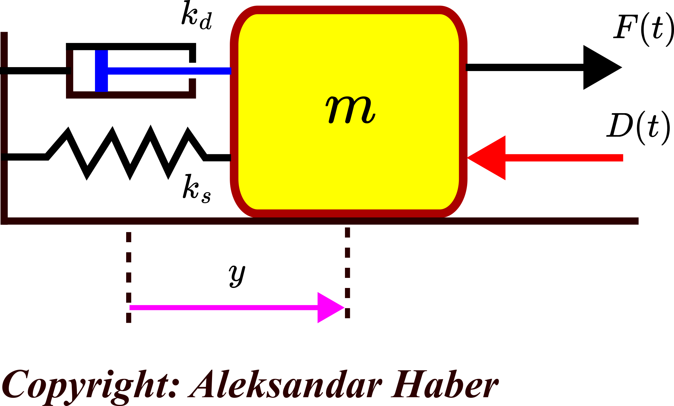
In this figure, ![]() and
and ![]() are spring and damping constants, respectively,
are spring and damping constants, respectively, ![]() is the control force (control input) calculated by the controller,
is the control force (control input) calculated by the controller, ![]() is the displacement of the mass from its equilibrium point, and
is the displacement of the mass from its equilibrium point, and ![]() is the disturbance force (external input disturbance) that acts on the system dynamics.
is the disturbance force (external input disturbance) that acts on the system dynamics. ![]() and
and ![]() are functions of time
are functions of time ![]() . The disturbance
. The disturbance ![]() has a unit of force and it can originate from a number of external sources.
has a unit of force and it can originate from a number of external sources. ![]() can be a stochastic force acting on the plant dynamics or can be a deterministic force. In addition,
can be a stochastic force acting on the plant dynamics or can be a deterministic force. In addition, ![]() can be a combination of stochastic and deterministic components, such as harmonic (periodic) force perturbed by a random signal.
can be a combination of stochastic and deterministic components, such as harmonic (periodic) force perturbed by a random signal.
In this particular example, the control objective can be to control the displacement ![]() , despite the effect of the external input disturbances
, despite the effect of the external input disturbances ![]() . That is, the goal is to control the position of the mass despite the effect of external disturbance forces.
. That is, the goal is to control the position of the mass despite the effect of external disturbance forces.
Besides external input disturbances, we also have internal input disturbances. Next, we provide an explanation and definition of internal input disturbances. For that purpose, let us write a model of the mass-spring-damper system. From Newton’s second law, we obtain an ordinary differential equation describing the dynamics of the system:
(1) ![]()
where ![]() and
and ![]() are the first and second time derivatives of the displacement
are the first and second time derivatives of the displacement ![]() . Let us now assume that a modeler and a control designer think that the model of the system looks like this:
. Let us now assume that a modeler and a control designer think that the model of the system looks like this:
(2) ![]()
That is, the system modeler and control designer think that the damping is not affecting the system. That is why they have omitted the damping in their model given by equation (2). However, in reality, the damping is affecting the model. After several model validation steps in which they compared the model with the experimental data, they came to the conclusion that something was missing in their model. To overcome this fact, they have included the damping term as an input disturbance. Namely, from (1), we have
(3) ![]()
The last equation can be written like this:
(4) ![]()
where ![]() is the internal input disturbance. Note that this input disturbance is actually dependent on the control signal. This is because the term
is the internal input disturbance. Note that this input disturbance is actually dependent on the control signal. This is because the term ![]() depends on the first derivative of the displacement, and displacement is controlled by the force
depends on the first derivative of the displacement, and displacement is controlled by the force ![]() that is determined by the control disturbance. This form of input disturbance comes from the lack of knowledge of the model structure. Model structure is the mathematical form of the model that includes all the terms, derivatives, and constants.
that is determined by the control disturbance. This form of input disturbance comes from the lack of knowledge of the model structure. Model structure is the mathematical form of the model that includes all the terms, derivatives, and constants.
However, there are also internal input disturbances that originate from the lack of knowledge of model parameters. To explain this, consider this scenario. Let us assume that our modelers and control engineers only know the nominal values of the model parameters. That is, let us assume the following
(5) 
where
 ,
,  , and
, and  are the exact values of the model parameters that match the physical reality perfectly. These values are called true model parameters. The true model parameters define the true model of the system which is almost never known exactly.
 ,
,  , and
, and  are the values of the model parameters that are used by the modeler and control designer. These parameters are usually called nominal parameters. The nominal model is determined by the nominal parameter values. That is, the nominal model is the model that is known to the system modeler and control engineer, and the nominal model is used to design a control algorithm. In fact, the true model is never known exactly!
 ,
,  , and
, and  are model uncertainties. That is, these variables represent a mismatch between the true and nominal model parameters, that is, they represent the mismatch between the true and nominal models.
By substituting (5) in (1), we obtain
(6) ![]()
After rearranging the last equation, we obtain
(7) ![]()
Next, we can define the internal input disturbance ![]()
(8) ![]()
Consequently, our dynamics can be written in the compact nominal form
(9) ![]()
The system modeler and control engineer can now work with the nominal model parameters ![]() , and
, and ![]() and they can consider the model uncertainties as disturbances. This is a very important technique and control-design philosophy in control engineering that is the basis of robust and data-driven control approaches.
and they can consider the model uncertainties as disturbances. This is a very important technique and control-design philosophy in control engineering that is the basis of robust and data-driven control approaches.
From the previous example, we can conclude that internal input disturbances can also originate from the lack of knowledge of the values of system parameters and not only from the lack of knowledge of the system structure. Another important thing to observe is that the internal input disturbances affect the nominal plant dynamics! That is, they are not physically present in our system, they originate from our modeling approach and the simplifications of the system dynamics. In fact, one can argue that every model is not an exact model, and that is why it is a good idea to include disturbances in our model to take into account unmodeled dynamics.
Definition of the internal input disturbances: the internal input disturbances are inputs that affect the nominal plant dynamics and that take into account our lack of knowledge of the numerical values of the model parameters and the lack of knowledge of the model structure.
Disturbance Observers – Basic Idea
The main motivation for introducing disturbance observers: Consider the control structure shown in the figure below.
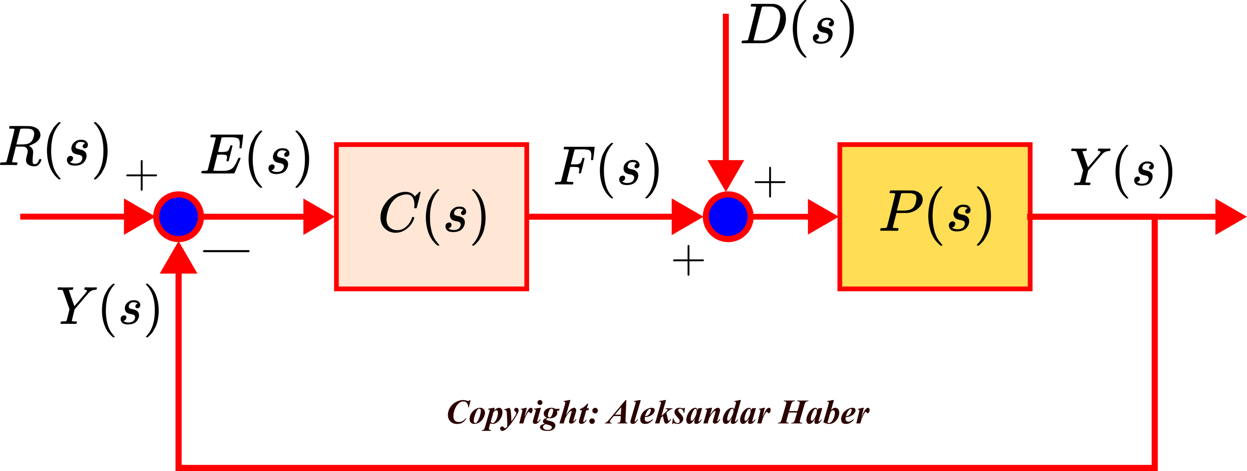
In the figure above:
 ,
,  , and
, and  are Laplace transforms of the system output (displacement)
  , input disturbance
  , and control input force
  , respectively.
  is the transfer function of the true system model (plant).
 is the transfer function of the control algorithm.
  is the Laplace transform of the reference signal
  . The control objective is to make sure that the output
  tracks the reference signal.
 is the control error in the Laplace domain. In the time domain, the error is
  .
.
Let us assume that the controller ![]() is a PID controller, that the plant is a second-order stable system, and that the disturbance is a constant signal. Then, due to the integral term, the PID controller will be able to suppress the constant disturbance. However, let us now assume that the disturbance is a harmonic signal, such as a sinusoidal signal. The PID controller cannot achieve a complete rejection and attenuation of this type of disturbance. This motivates us to introduce a disturbance observer. The disturbance observer will be able to estimate the disturbance and suppress it. Let us introduce a concrete example that illustrates the limitations of the PID controller for suppressing non-constant disturbances. Consider the following system
is a PID controller, that the plant is a second-order stable system, and that the disturbance is a constant signal. Then, due to the integral term, the PID controller will be able to suppress the constant disturbance. However, let us now assume that the disturbance is a harmonic signal, such as a sinusoidal signal. The PID controller cannot achieve a complete rejection and attenuation of this type of disturbance. This motivates us to introduce a disturbance observer. The disturbance observer will be able to estimate the disturbance and suppress it. Let us introduce a concrete example that illustrates the limitations of the PID controller for suppressing non-constant disturbances. Consider the following system
(10) ![]()
with the PID controller with the following parameters: proportional gain ![]() , integral gain
, integral gain ![]() , and the derivative gain
, and the derivative gain ![]() . Let us assume a constant disturbance signal
. Let us assume a constant disturbance signal ![]() and a reference signal
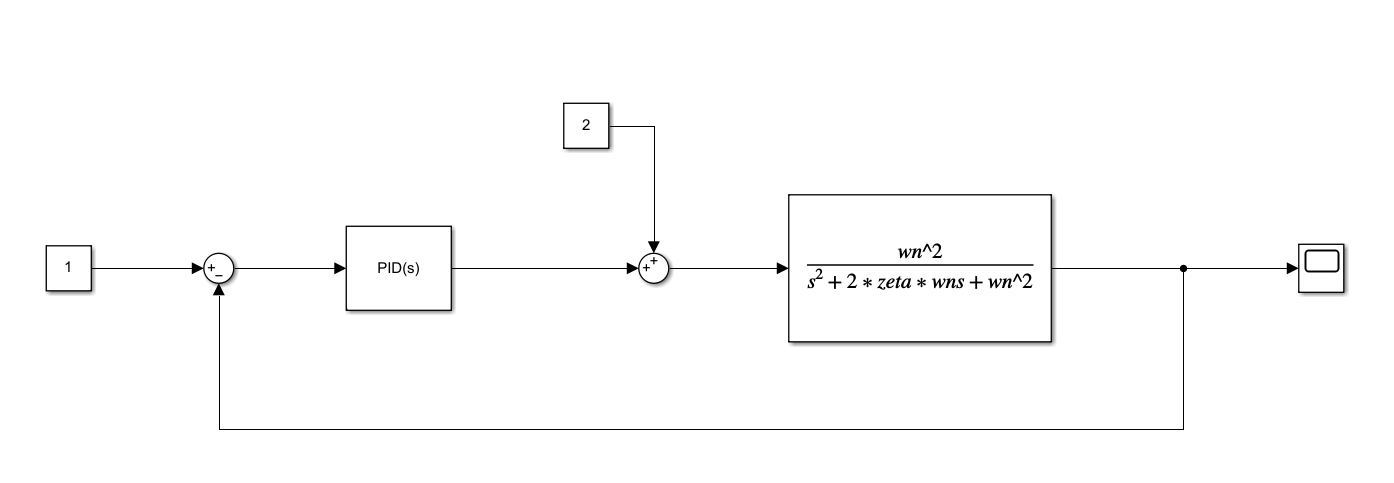
and a reference signal ![]() . The Simulink block diagram is shown below.
. The Simulink block diagram is shown below.
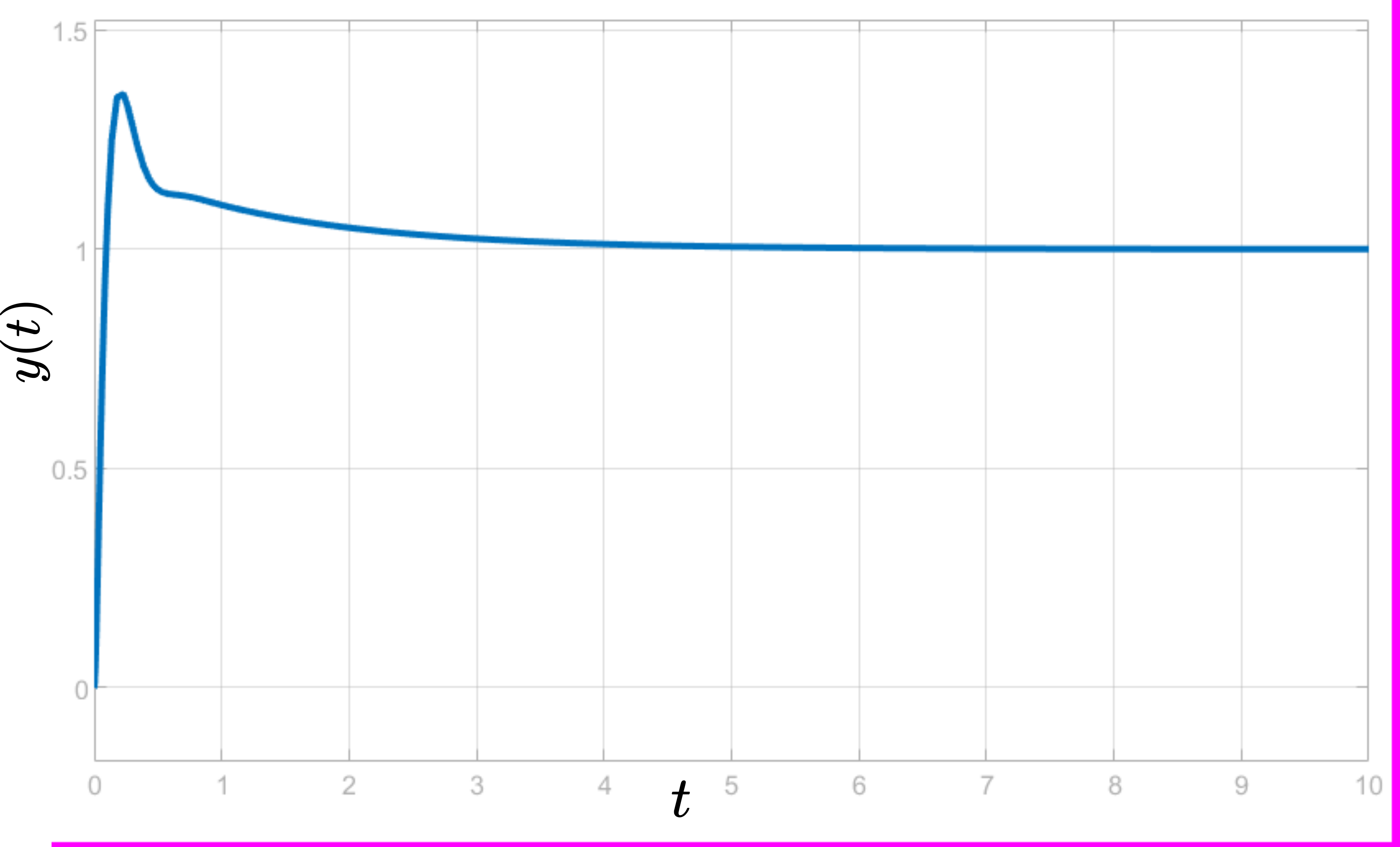
The control results are shown below. The figure below shows the controlled output ![]() as a function of time
as a function of time ![]() . We can observe that the controller is able to suppress constant disturbances.
. We can observe that the controller is able to suppress constant disturbances.
Now, let us change the configuration of the system, and let us introduce harmonic disturbances having the following form ![]() . The modified Simulink block diagram is shown below.
. The modified Simulink block diagram is shown below.
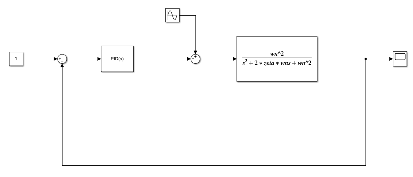
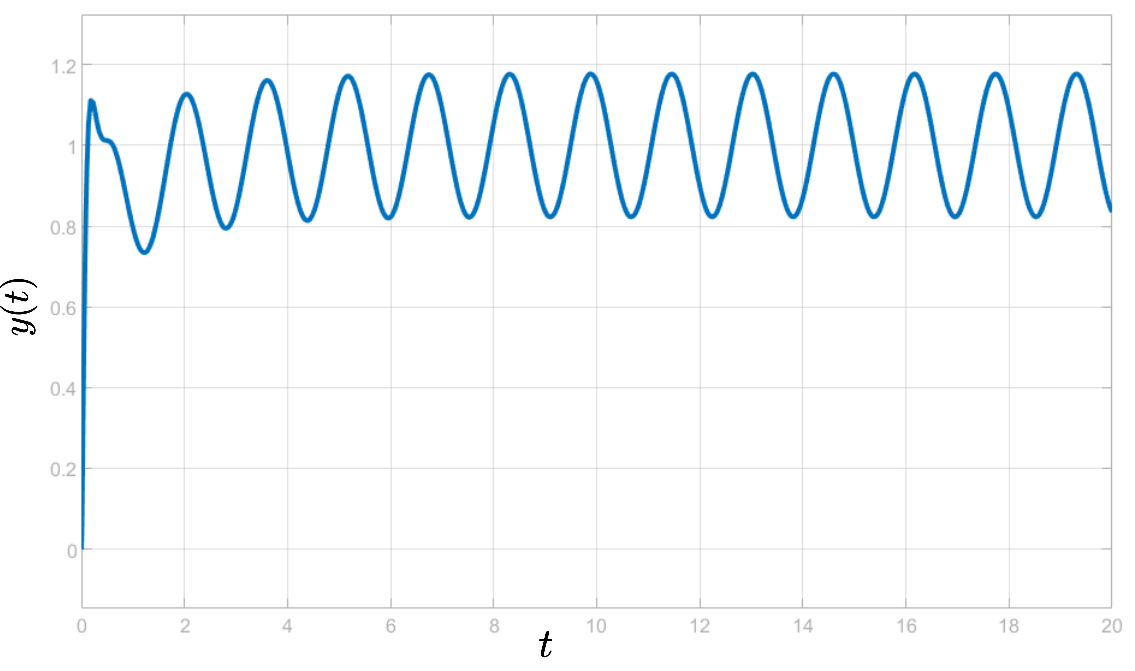
The control results are shown in the figure below. This figure shows ![]() as the function of time
as the function of time ![]() . As can clearly be observed from the figure below, the pure PID control algorithm is not able to reject the harmonic disturbances.
. As can clearly be observed from the figure below, the pure PID control algorithm is not able to reject the harmonic disturbances.
The previous discussion and the example motivate us to introduce the disturbance observer. The main idea of the disturbance observer is graphically illustrated in the figure below.
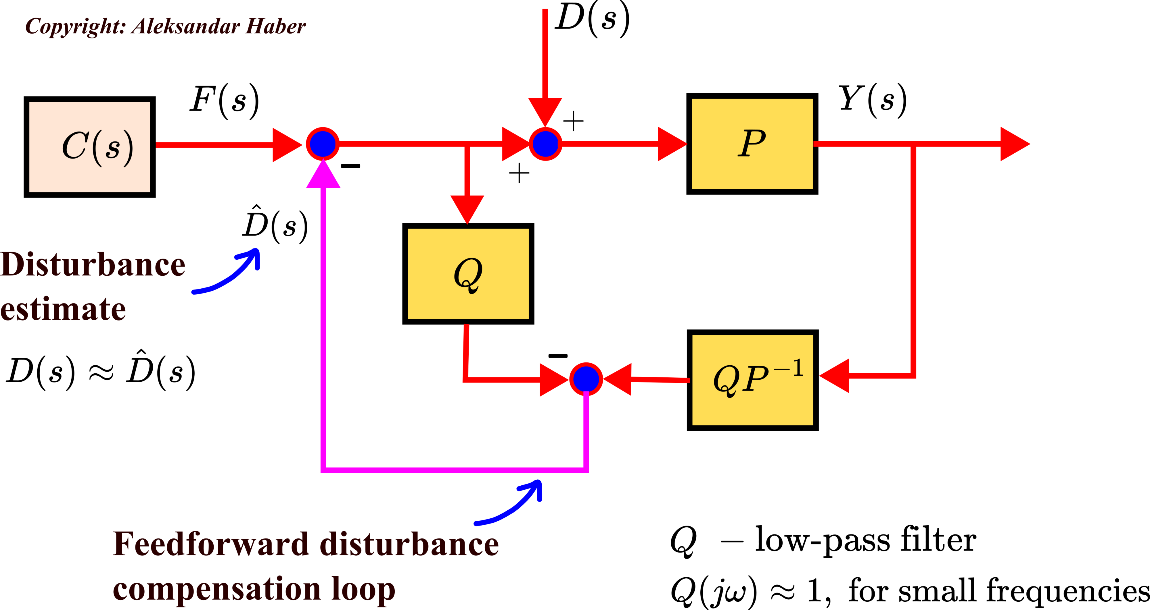
In the above figure, ![]() is a transfer function of a low-pass filter that is a design parameter and selected by the user.
is a transfer function of a low-pass filter that is a design parameter and selected by the user. ![]() is an inverse of the transfer function
is an inverse of the transfer function ![]() . The main idea of the disturbance observer is to introduce a feedforward disturbance compensation loop that will cancel the disturbance
. The main idea of the disturbance observer is to introduce a feedforward disturbance compensation loop that will cancel the disturbance ![]() . This is achieved by estimating the disturbance. The estimate of the disturbance is denoted by
. This is achieved by estimating the disturbance. The estimate of the disturbance is denoted by ![]() . In the sequel, we explain how disturbance observer works.
. In the sequel, we explain how disturbance observer works.
First of all, the filter ![]() should be selected as a low-pass filter that satisfies the following property:
should be selected as a low-pass filter that satisfies the following property:
(11) ![]()
where ![]() is obtained by substituting
is obtained by substituting ![]() by
by ![]() in
in ![]() .
.
Then, the filter ![]() should be selected such that the relative degree should be greater than or equal to the relative degree of the nominal transfer function
should be selected such that the relative degree should be greater than or equal to the relative degree of the nominal transfer function ![]() . The relative degree of a transfer function is a difference between the order of the polynomial in the denominator and the order of the polynomial in the numerator of the transfer function. For example, the model in (10) has the relative degree of
. The relative degree of a transfer function is a difference between the order of the polynomial in the denominator and the order of the polynomial in the numerator of the transfer function. For example, the model in (10) has the relative degree of ![]() . This means that the relative degree of the Q filter should be at least 2. The reason for this is to make sure that the transfer function product
. This means that the relative degree of the Q filter should be at least 2. The reason for this is to make sure that the transfer function product
(12) ![]()
is a proper transfer function. That is, this transfer function product should be realizable. See the example at the end of this tutorial to see the form of the filter ![]() for the second-order system.
for the second-order system.
Due to (11), for small (radial) frequencies ![]() , the above block diagram and the control system essentially looks like this:
, the above block diagram and the control system essentially looks like this:
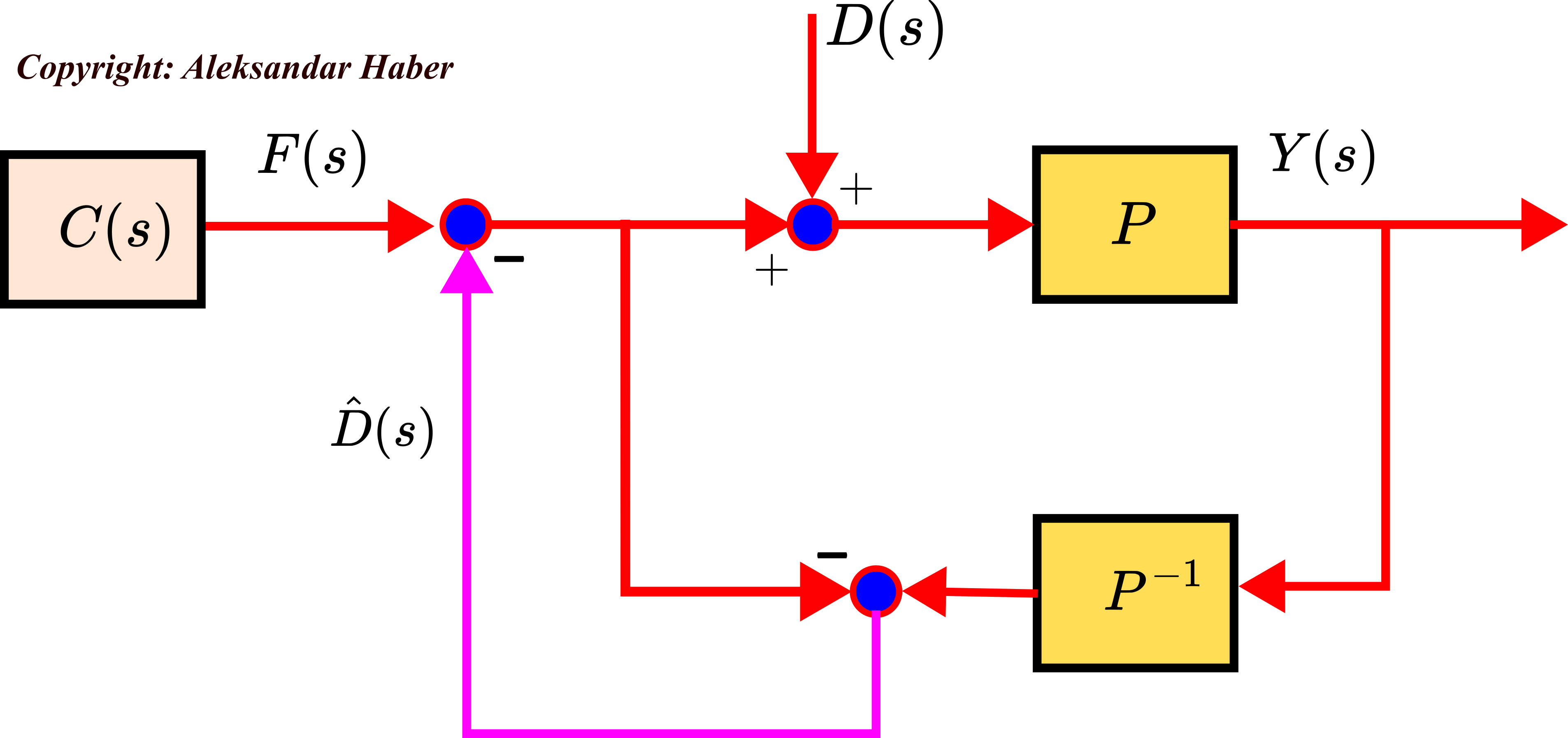
Let us assume that ![]() , that is, let us assume that the disturbance is accurately estimated. Then, from the last figure, we obtain the following diagram
, that is, let us assume that the disturbance is accurately estimated. Then, from the last figure, we obtain the following diagram
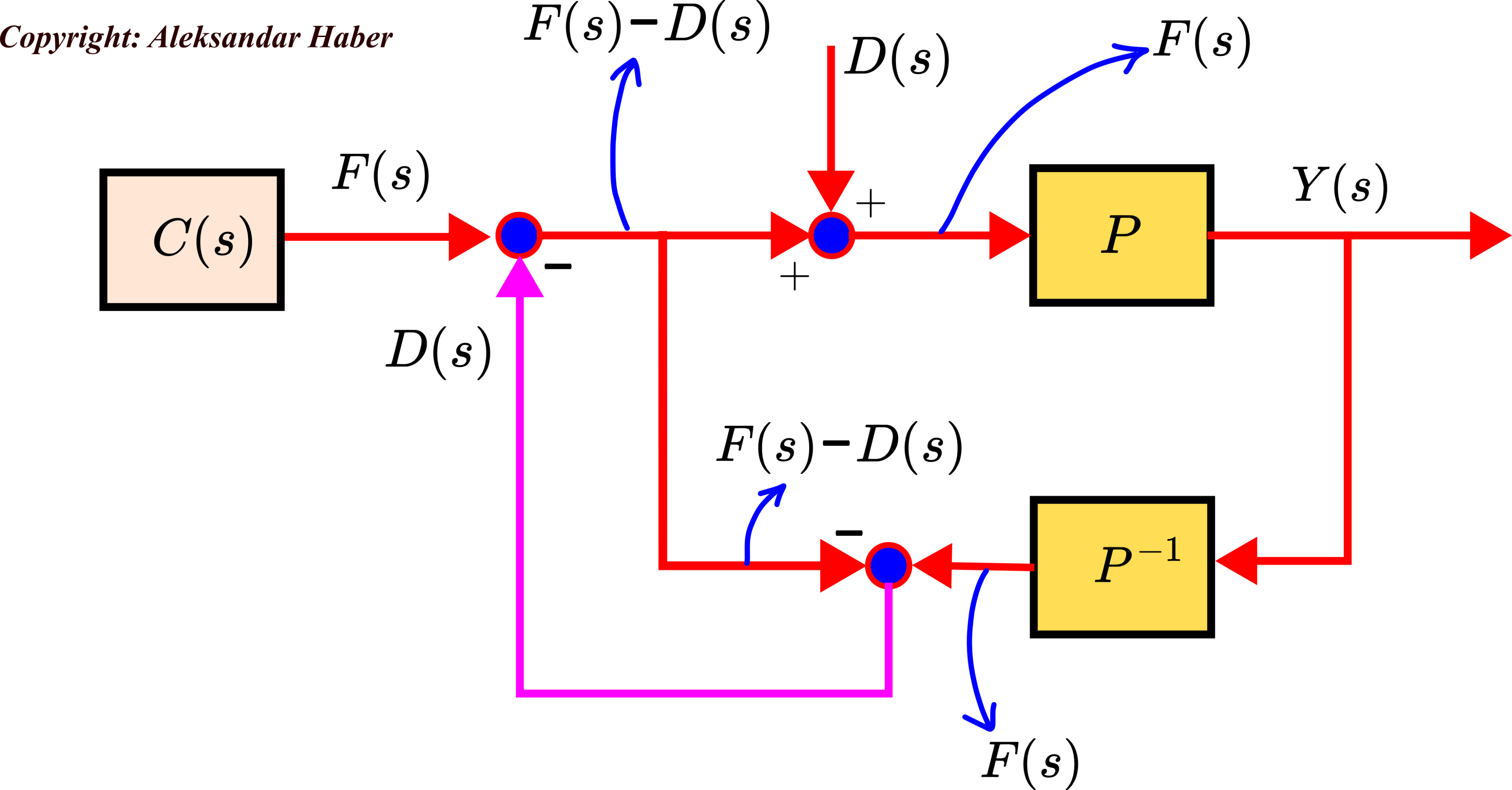
By inverting the plant transfer function ![]() , and by feeding the output of the system
, and by feeding the output of the system ![]() to the inverted plant, we obtain the control input
to the inverted plant, we obtain the control input ![]() . This control input is then added to the term
. This control input is then added to the term ![]() . In this way, we obtain
. In this way, we obtain ![]() . Then
. Then ![]() is sent as a feedforward signal and added to the control input
is sent as a feedforward signal and added to the control input ![]() that is calculated by the controller
that is calculated by the controller ![]() . The result is
. The result is ![]() . This signal directly cancels the disturbance
. This signal directly cancels the disturbance ![]() . Consequently, we only have the control input
. Consequently, we only have the control input ![]() that affects the plant. In this way, we reject the disturbances.
that affects the plant. In this way, we reject the disturbances.
However, the figure above is an idealization of the real block diagram. The estimate ![]() is almost never exactly equal to the true value of disturbance. Also, in the above block diagrams, we assumed that the model of the plant is known accurately. In fact, we only know the nominal model and the nominal transfer function, which is denoted by
is almost never exactly equal to the true value of disturbance. Also, in the above block diagrams, we assumed that the model of the plant is known accurately. In fact, we only know the nominal model and the nominal transfer function, which is denoted by ![]() . The complete feedback control algorithm is given below.
. The complete feedback control algorithm is given below.
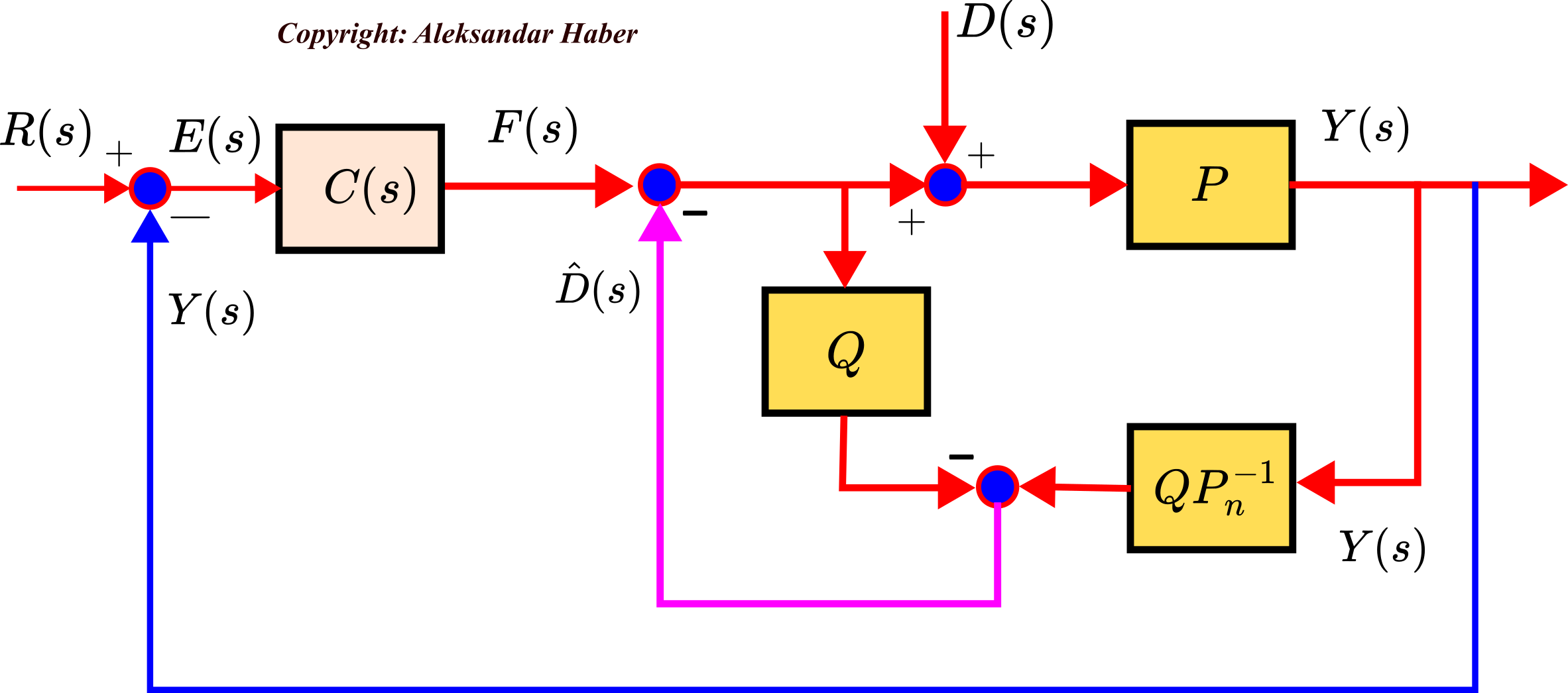
Our goal is to derive the transfer functions of the model that provide more insights into how the disturbance observer works in practice. From the above figure, we have
(13) 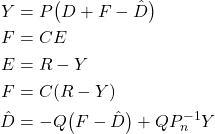
From the last set of equations, we have
(14) ![]()
From the equations in (13) and from (14), we obtain
(15) ![]()
where the input-to-output transfer function ![]() and disturbance-to-output transfer function
and disturbance-to-output transfer function ![]() have the following forms
have the following forms
(16) 
The filter ![]() is selected as a low-pass filter with the following property
is selected as a low-pass filter with the following property
(17) ![]()
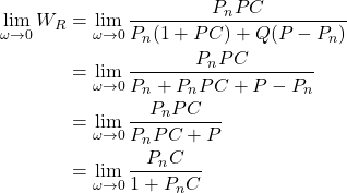
Taking into account this property, we have
(18) 
On the other hand,
(19) ![]()
Consequently, we conclude
- From (18) it follows that for low frequencies or asymptotically the closed-loop system with the disturbance observer behaves like a closed-loop system formed on the basis of the nominal plant. This is because the closed-loop transfer function from the reference signal to the output for the nominal plant is:
(20)

In this way, we are able to control the system accurately despite the presence of the model mismatch between the nominal model and the true model. That is, if the controller is designed on the basis of the nominal model
  , then for low frequencies or asymptotically this controller will be able to control the true system represented by the transfer function
  as accurately as controlling the nominal model.
 - From (19) we conclude that for low frequencies or asymptotically, the disturbance observer is able to attenuate the effects of disturbances.
A disturbance observer can estimate disturbances accurately if disturbance frequencies are in the bandwidth range of the low-pass Q filter. Consequently, the bandwidth of the Q-filter should be set as high as possible. This is not always possible and can produce negative effects in the presence of strong measurement noise.
Example of Controlling the System Using Disturbance Observer
We have created a video tutorial explaining how to simulate the disturbance observer in Simulink. The tutorial is given below.
For comparison with a pure PID control approach, let us use the previous example that is used to illustrate the limitations of a pure PID control algorithm. The true model is given by
(21) ![]()
The controller is a PID controller with the following parameters: proportional gain ![]() , integral gain
, integral gain ![]() , and the derivative gain
, and the derivative gain ![]() . Let us assume a harmonic disturbance signal
. Let us assume a harmonic disturbance signal ![]() and a constant reference signal
and a constant reference signal ![]() that we want to track. To make the simulation realistic, we assume the nominal model that is different from the true model. That is, we assume that we do not know the true model exactly. The nominal transfer function is given by
that we want to track. To make the simulation realistic, we assume the nominal model that is different from the true model. That is, we assume that we do not know the true model exactly. The nominal transfer function is given by
(22) ![]()
The Q filter is given by
(23) ![]()
The product ![]() is
is
(24) ![]()
Consequently, this product is a proper function and thus realizable.
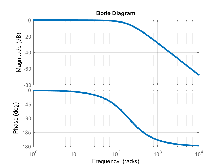
The Bode diagram of the Q filter is given below.
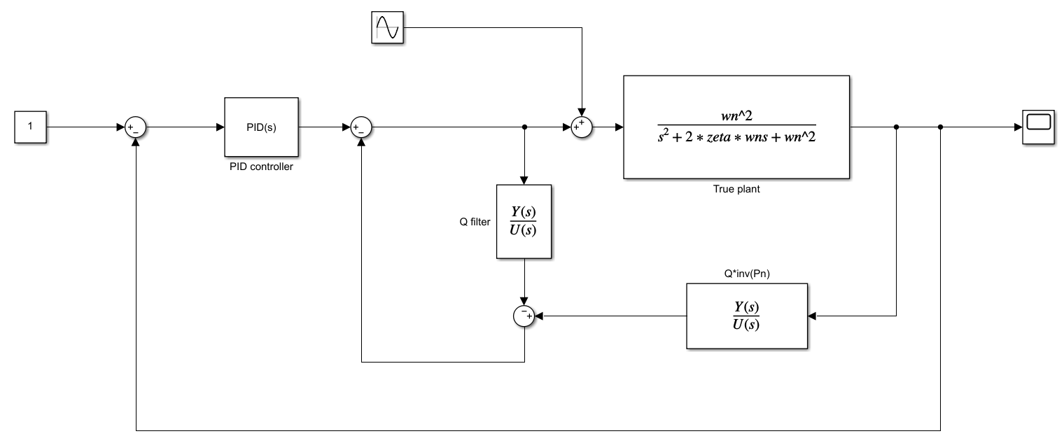
The Simulink block diagram of the disturbance observer and the control algorithm is shown below.
The control results are shown below. The figure below shows the controlled output ![]() of the system as a function of time.
of the system as a function of time.
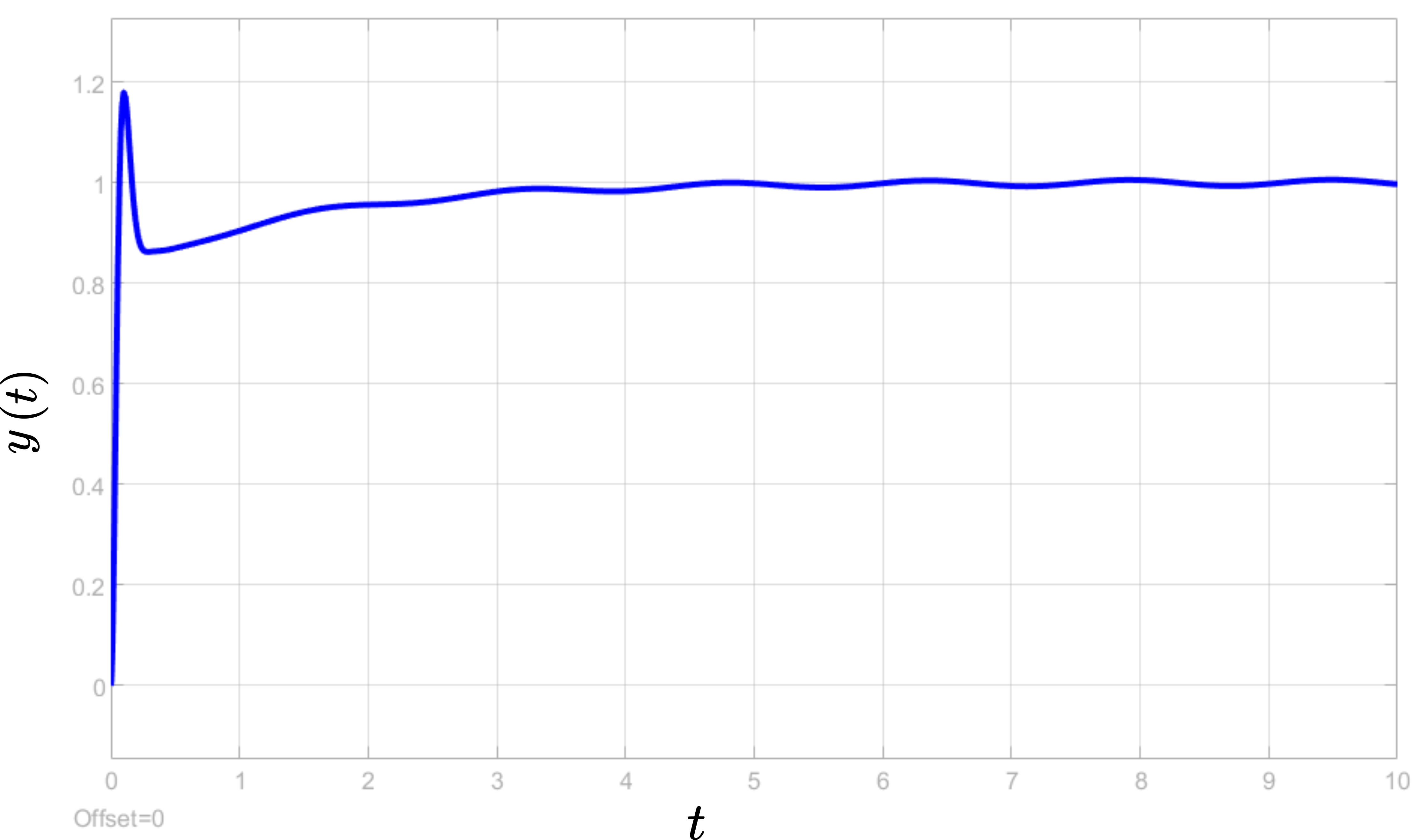
From the above figure, we can see that the disturbance observer together with the PID controller is capable of almost completely rejecting the harmonic disturbances. By comparing these results with the results shown in Fig. 6 that show the performance of the pure PID controller, we can clearly observe the advantages of disturbance observer compared to pure PID control algorithm.