In this control theory and control engineering tutorial, we provide a brief introduction to disturbance observers and controllers that are based on disturbance observers. The field of disturbance observers is well-developed and it is challenging and time-consuming to explain all the caveats of disturbance observers. Instead, in this tutorial, we provide an intuitive explanation of disturbance observers that can serve as a starting point for a deeper study of disturbance observers. We briefly explain the mathematics behind disturbance observers and why disturbance observers work in practice. In the YouTube tutorials we explain how to implement disturbance observers in MATLAB and Simulink. The YouTube tutorials are given below.


What are Disturbances in Control Engineering?
There are a large number of disturbances that can affect the dynamics of the system. Consequently, there are different classifications of disturbances. In this tutorial, we focus on the input disturbances in the context of presenting the main ideas of the disturbance observers. That is, we focus on the disturbances that affect the plant dynamics through the input signals. There are also disturbances that affect the output of the system. Finally, we also have disturbances that do not affect inputs and outputs, but instead, that affect some other signals in a feedback control system.
Let us first define external input disturbances.
Definition of external input disturbances: External input disturbances are external inputs that affect the dynamics of the system (plant dynamics) and that are not created by the controller. That is, external input disturbances are inputs to the plant that are different from the control inputs. The external input disturbances are usually not known or we only have limited knowledge about certain aspects of external input disturbances. We are not able to actively control external input disturbances at their source.
Let us now give a practical example of the external input disturbances. Consider a mass-spring-damper system shown below.

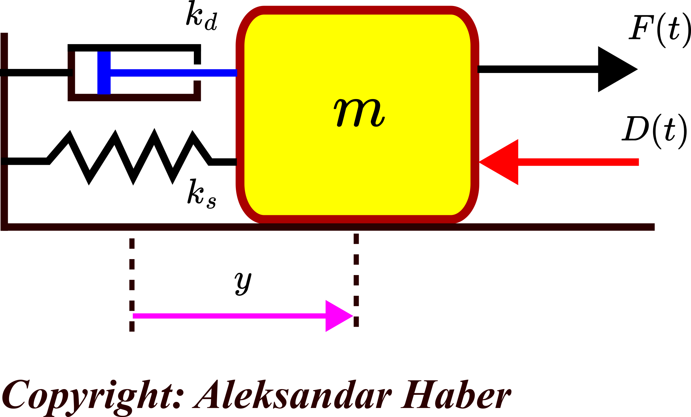
In this figure, 


In this particular example, the control objective can be to control the displacement
Besides external input disturbances, we also have internal input disturbances. Next, we provide an explanation and definition of internal input disturbances. For that purpose, let us write a model of the mass-spring-damper system. From Newton’s second law, we obtain an ordinary differential equation describing the dynamics of the system:
(1) 

where 


(2) 

That is, the system modeler and control designer think that the damping is not affecting the system. That is why they have omitted the damping in their model given by equation (2). However, in reality, the damping is affecting the model. After several model validation steps in which they compared the model with the experimental data, they came to the conclusion that something was missing in their model. To overcome this fact, they have included the damping term as an input disturbance. Namely, from (1), we have
(3) 

The last equation can be written like this:
(4) 

where 


However, there are also internal input disturbances that originate from the lack of knowledge of model parameters. To explain this, consider this scenario. Let us assume that our modelers and control engineers only know the nominal values of the model parameters. That is, let us assume the following
(5) 

where


By substituting (5) in (1), we obtain
(6) 

After rearranging the last equation, we obtain
(7) 

Next, we can define the internal input disturbance 
(8) 

Consequently, our dynamics can be written in the compact nominal form
(9) 

The system modeler and control engineer can now work with the nominal model parameters 

From the previous example, we can conclude that internal input disturbances can also originate from the lack of knowledge of the values of system parameters and not only from the lack of knowledge of the system structure. Another important thing to observe is that the internal input disturbances affect the nominal plant dynamics! That is, they are not physically present in our system, they originate from our modeling approach and the simplifications of the system dynamics. In fact, one can argue that every model is not an exact model, and that is why it is a good idea to include disturbances in our model to take into account unmodeled dynamics.
Definition of the internal input disturbances: the internal input disturbances are inputs that affect the nominal plant dynamics and that take into account our lack of knowledge of the numerical values of the model parameters and the lack of knowledge of the model structure.
Disturbance Observers – Basic Idea
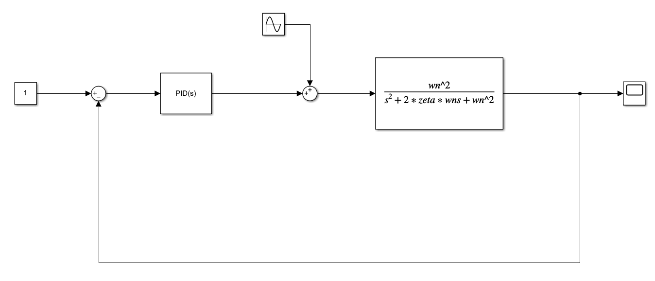
The main motivation for introducing disturbance observers: Consider the control structure shown in the figure below.

In the figure above:


Let us assume that the controller
(10) 

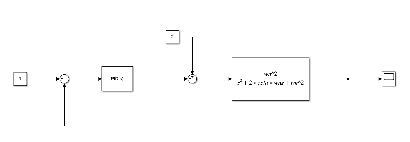
with the PID controller with the following parameters: proportional gain 


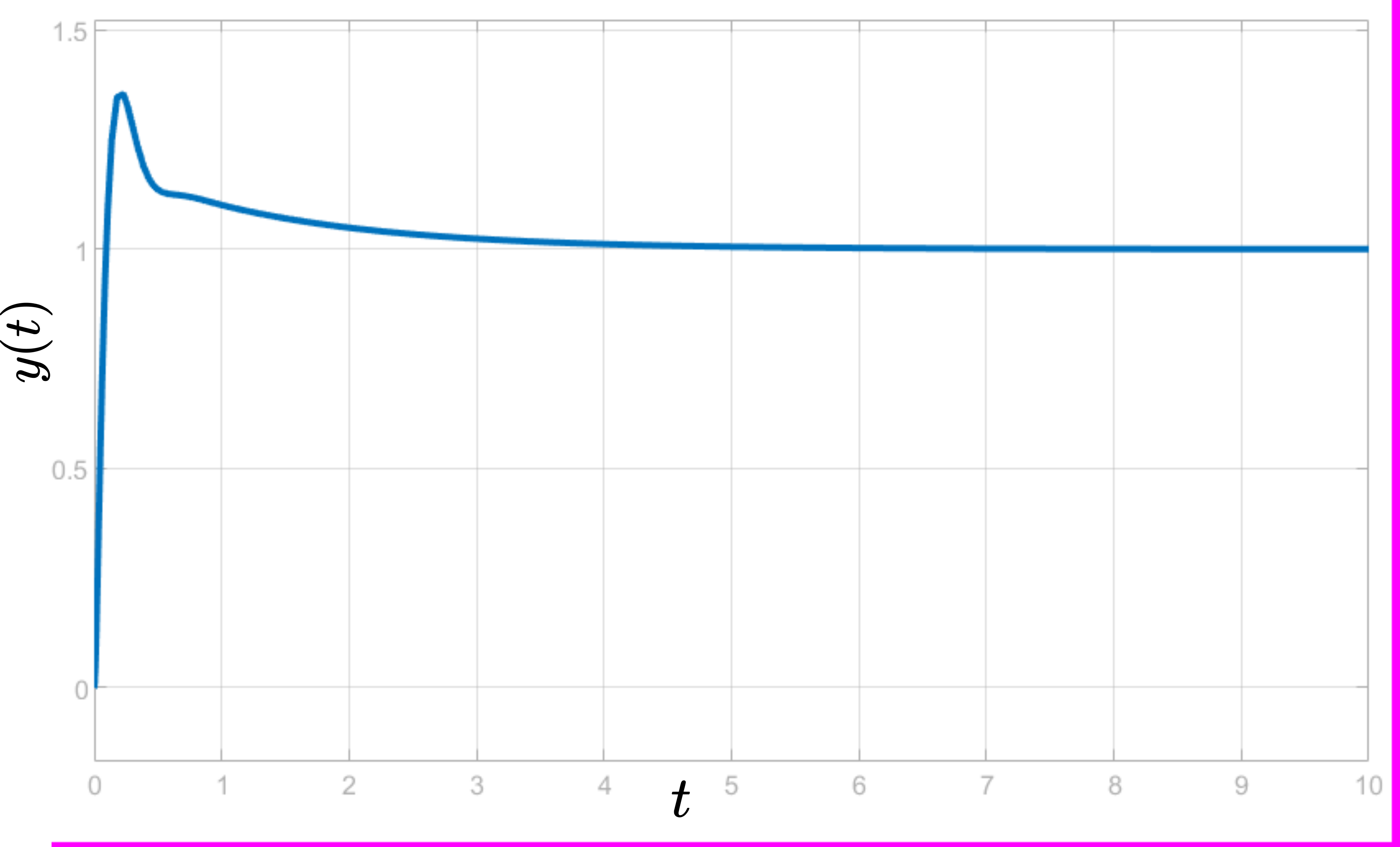
The control results are shown below. The figure below shows the controlled output

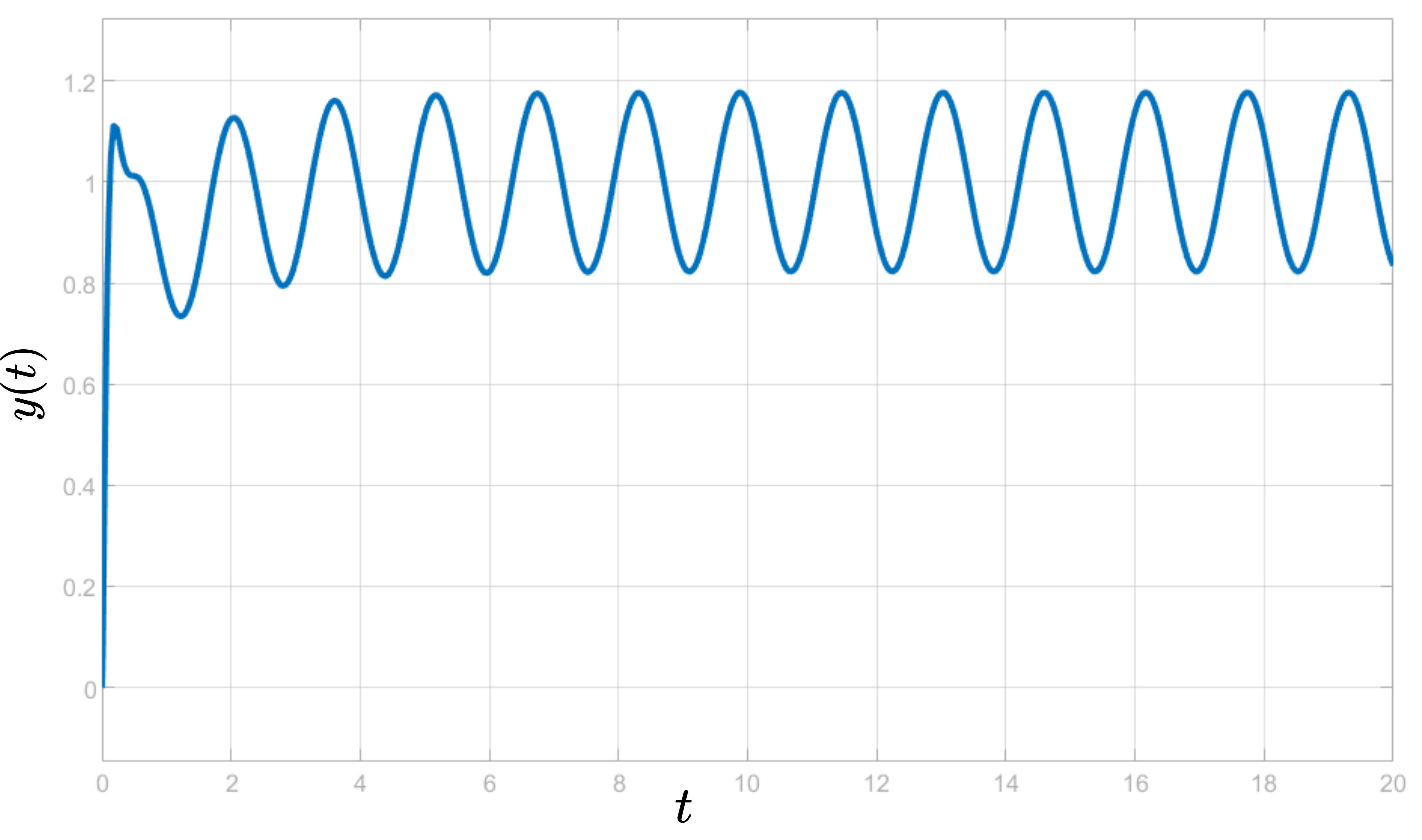
Now, let us change the configuration of the system, and let us introduce harmonic disturbances having the following form 


The control results are shown in the figure below. This figure shows

The previous discussion and the example motivate us to introduce the disturbance observer. The main idea of the disturbance observer is graphically illustrated in the figure below.

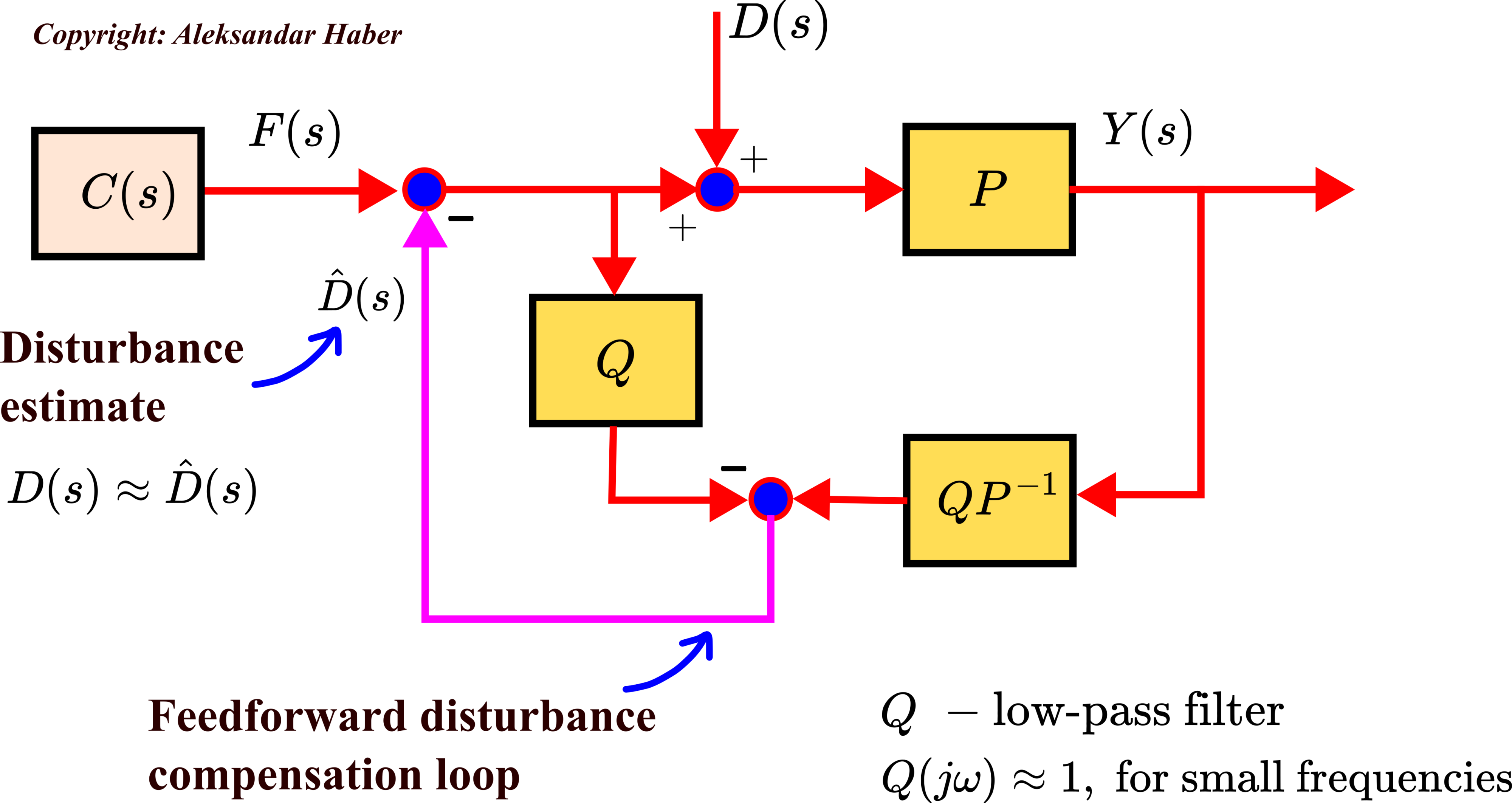
In the above figure, 


First of all, the filter 
(11) 

where 


Then, the filter 


(12) 

is a proper transfer function. That is, this transfer function product should be realizable. See the example at the end of this tutorial to see the form of the filter
Due to (11), for small (radial) frequencies 


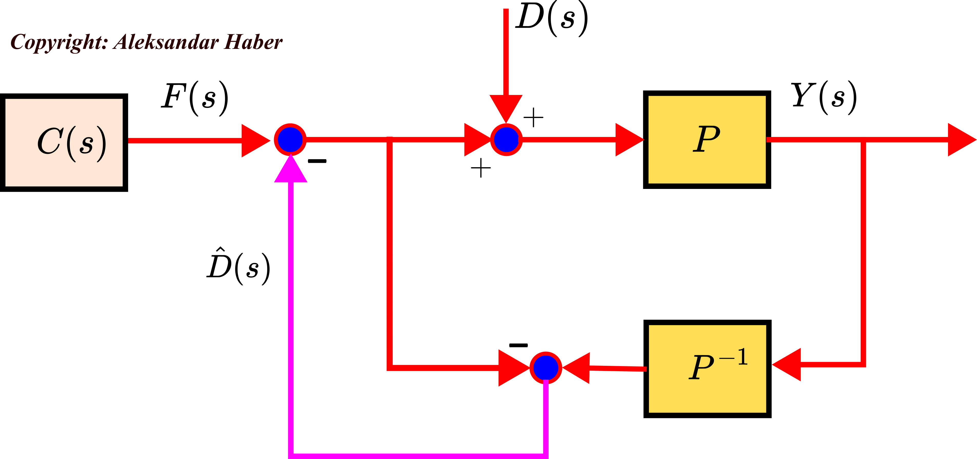
Let us assume that 


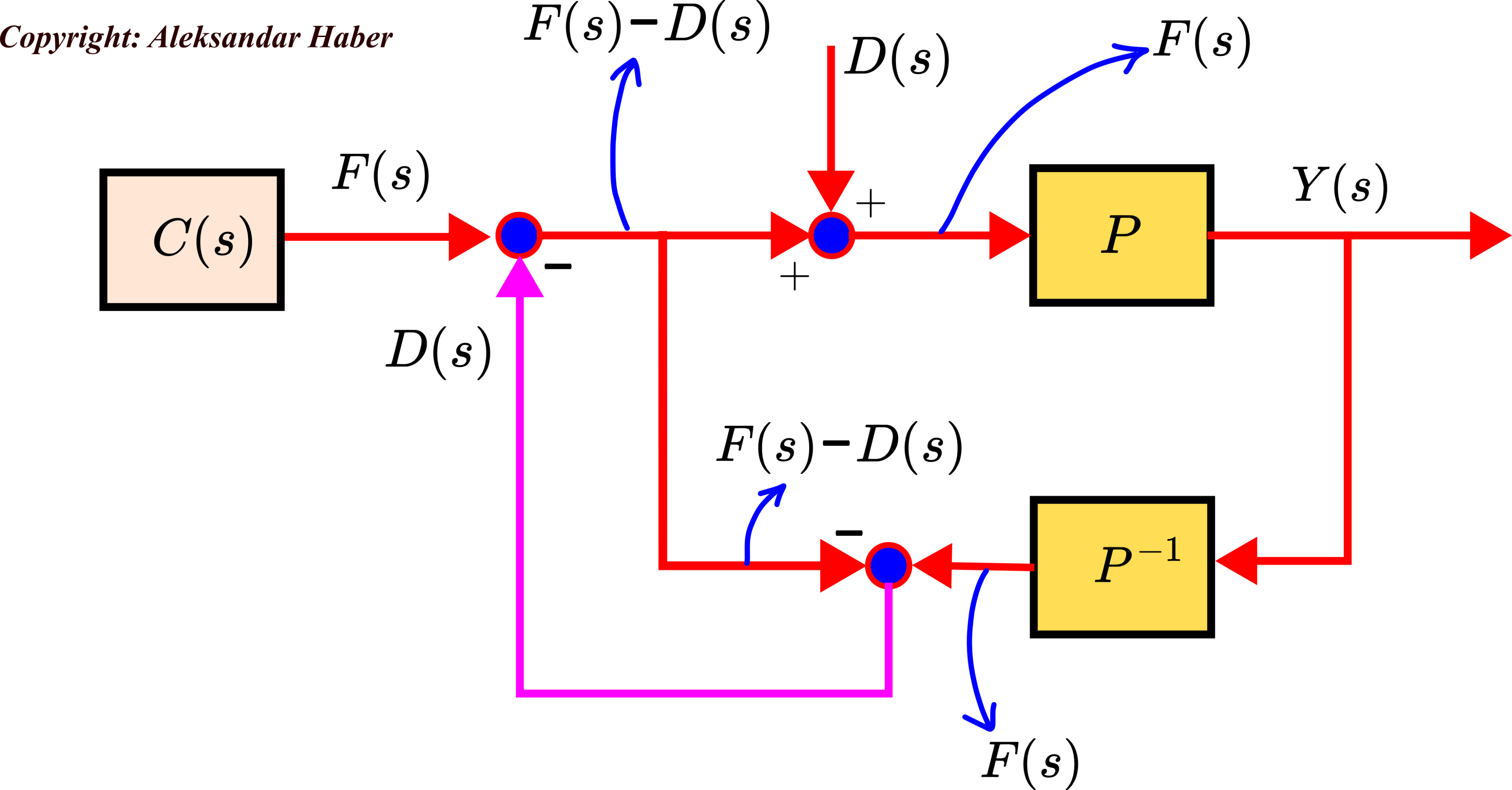
By inverting the plant transfer function 


However, the figure above is an idealization of the real block diagram. The estimate 


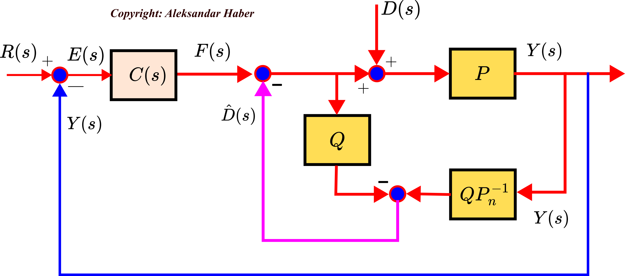
Our goal is to derive the transfer functions of the model that provide more insights into how the disturbance observer works in practice. From the above figure, we have
(13) 

From the last set of equations, we have
(14) 

From the equations in (13) and from (14), we obtain
(15) 

where the input-to-output transfer function 


(16) 

The filter
(17) 
Taking into account this property, we have
(18) 

On the other hand,
(19) 

Consequently, we conclude
- From (18) it follows that for low frequencies or asymptotically the closed-loop system with the disturbance observer behaves like a closed-loop system formed on the basis of the nominal plant. This is because the closed-loop transfer function from the reference signal to the output for the nominal plant is:
(20)

In this way, we are able to control the system accurately despite the presence of the model mismatch between the nominal model and the true model. That is, if the controller - From (19) we conclude that for low frequencies or asymptotically, the disturbance observer is able to attenuate the effects of disturbances.

A disturbance observer can estimate disturbances accurately if disturbance frequencies are in the bandwidth range of the low-pass Q filter. Consequently, the bandwidth of the Q-filter should be set as high as possible. This is not always possible and can produce negative effects in the presence of strong measurement noise.
Example of Controlling the System Using Disturbance Observer
We have created a video tutorial explaining how to simulate the disturbance observer in Simulink. The tutorial is given below.
For comparison with a pure PID control approach, let us use the previous example that is used to illustrate the limitations of a pure PID control algorithm. The true model is given by
(21) 
The controller is a PID controller with the following parameters: proportional gain
(22) 

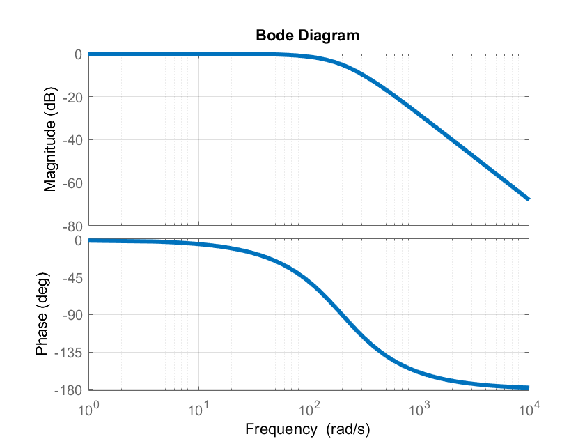
The Q filter is given by
(23) 

The product 

(24) 

Consequently, this product is a proper function and thus realizable.
The Bode diagram of the Q filter is given below.

The Simulink block diagram of the disturbance observer and the control algorithm is shown below.

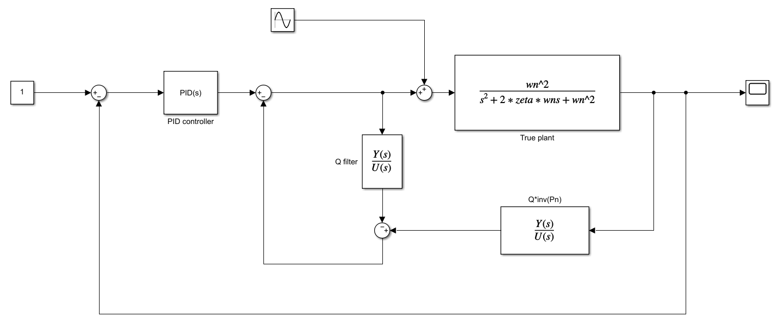
The control results are shown below. The figure below shows the controlled output

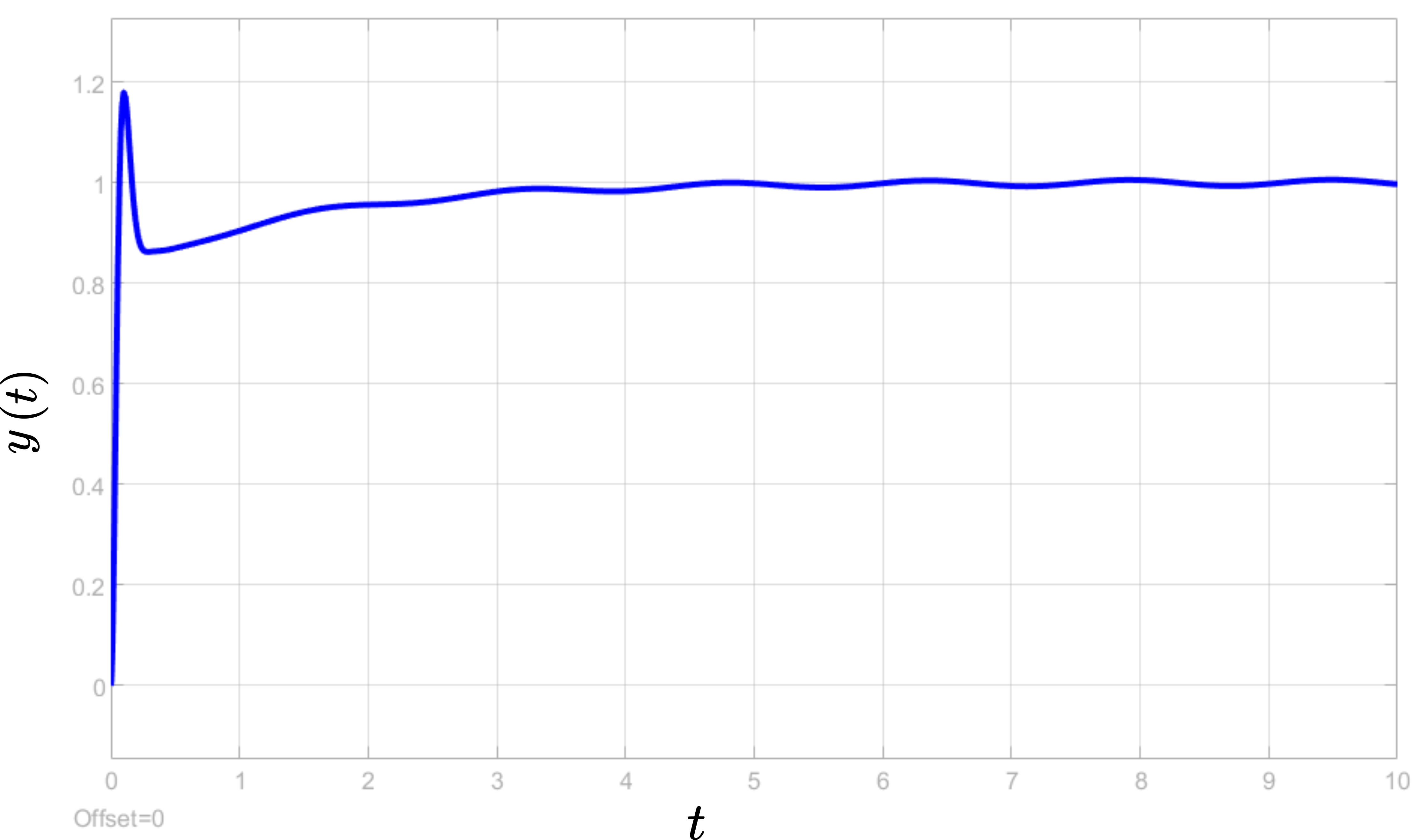
From the above figure, we can see that the disturbance observer together with the PID controller is capable of almost completely rejecting the harmonic disturbances. By comparing these results with the results shown in Fig. 6 that show the performance of the pure PID controller, we can clearly observe the advantages of disturbance observer compared to pure PID control algorithm.