Tutorial on Solving Linear Programming (Linear Optimization) Problems in MATLAB – Fusion of Engineering, Control, Coding, Machine Learning, and Science

In this post, we explain how to solve linear programming problems in MATLAB. The YouTube video accompanying this post is given below.

Formulation of Linear Programming Problems in MATLAB

To solve linear programming problems in MATLAB you need the Optimization Toolbox.

In MATLAB, linear programming problems are formulated as follows

(1) $\begin{align*}& \min_{\mathbf{x}} \mathbf{f}^{T} \mathbf{x} \\& \text{subject to:} \;\; \\& A\cdot \mathbf{x} \le \mathbf{b} \\& A_{\text{eq}}\cdot \mathbf{x} =\mathbf{b}_{\text{eq}} \\& \mathbf{l}_{b} \le \mathbf{x} \le \mathbf{u}_{b}\end{align*}$

where $\mathbf{f}$ is the vector of coefficients, $\mathbf{x}$ is the vector of optimization variables, $A$ is the matrix of coefficients describing the inequality constraints, $A_{\text{eq}}$ is the matrix defining the equality constraints, and $\mathbf{b}$ , $\mathbf{b}_{\text{eq}}$ , $\mathbf{l}_{b}$ , and $\mathbf{u}_{b}$ are vectors of coefficients. The relation symbol $\le$ in (1) is applied element-wise, for example for the vector

(2) $\begin{align*}\mathbf{x}=\begin{bmatrix}x_{1} \\ x_{2} \end{bmatrix}\end{align*}$

the notation

(3) $\begin{align*}\begin{bmatrix} -1 \\ -2 \end{bmatrix} \le \mathbf{x} \le \begin{bmatrix} 1 \\ 2 \end{bmatrix}\end{align*}$

means

(4) $\begin{align*}-1\le x_{1} \le 1 \\-2\le x_{2} \le 2\end{align*}$

The cost function is defined by the scalar variable

(5) $\begin{align*}\mathbf{f}^{T} \mathbf{x}\end{align*}$

The problem (1) is called linear optimization or linear programming problems, because

1.) Cost function (5) is linear.
2.) The equality and inequality constraints are represented by linear functions.

This problem formulation is very similar to the standard formulation of linear programs. The main difference is that in standard form minimization in (1) is replaced by maximization.

Example of Transforming an Optimization Problem into the MATLAB Form

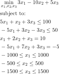
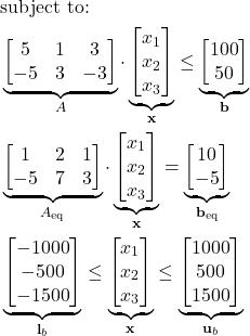
Here, we explain how to transform an optimization problem into the MATLAB form (1). Consider the following optimization problem

(6) $\begin{align*}& \min_{x_{1},x_{2},x_{3}} 3x_{1}-10x_{2}+5x_{3} \\& \text{subject to:} \;\; \\& 5x_{1}+x_{2}+3x_{3}\le 100 \\& -5x_{1}+3x_{2}-3x_{3}\le 50 \\& x_{1}+2x_{2}+x_{3}=10\\& -5x_{1}+7x_{2}+3x_{3}=-5 \\& -1000 \le x_{1}\le 1000 \\& -500 \le x_{2}\le 500 \\& -1500 \le x_{3}\le 1500\end{align*}$

We can write this problem as follows

(7) $\begin{align*}& \min_{\mathbf{x}} \underbrace{\begin{bmatrix}3 & -10 & 5\end{bmatrix}}_{\mathbf{f}^{T}} \cdot \underbrace{\begin{bmatrix} x_{1}\\ x_{2}\\ x_{3} \end{bmatrix}}_{\mathbf{x}} \end{align*}$

(8) $\begin{align*}& \text{subject to:} \\& \underbrace{\begin{bmatrix} 5 & 1 & 3 \\ -5 & 3 & -3 \end{bmatrix}}_{A} \cdot \underbrace{\begin{bmatrix} x_{1} \\ x_{2} \\ x_{3} \end{bmatrix}}_{\mathbf{x}} \le \underbrace{\begin{bmatrix}100 \\ 50 \end{bmatrix}}_{\mathbf{b}} \\& \underbrace{\begin{bmatrix} 1 & 2 & 1\\ -5 & 7 & 3 \end{bmatrix}}_{A_{\text{eq}}} \cdot \underbrace{\begin{bmatrix} x_{1} \\ x_{2} \\ x_{3} \end{bmatrix}}_{\mathbf{x}} = \underbrace{\begin{bmatrix} 10 \\ -5 \end{bmatrix}}_{\mathbf{b}_{\text{eq}}}\\& \underbrace{\begin{bmatrix} -1000 \\ -500 \\ -1500 \end{bmatrix}}_{\mathbf{l}_{b}} \le \underbrace{\begin{bmatrix} x_{1} \\ x_{2} \\ x_{3} \end{bmatrix}}_{\mathbf{x}} \le \underbrace{\begin{bmatrix} 1000 \\ 500 \\ 1500\end{bmatrix}}_{\mathbf{u}_{b}} \end{align*}$

Implementation in MATLAB

The optimization problem is defined and implemented in the MATLAB script below.

clear

f=[3 -10 5];
A=[5 1 4; -5 3 -3];
b=[100; 50];
Aeq=[1 2 1; -5 7 3];
beq=[10; -5];
lb=[-1000; -500; -1500];
ub=[1000; 500; 1500];


options = optimoptions('linprog','Algorithm','interior-point','Display','iter','MaxIterations',2000,'OptimalityTolerance',1e-9,'ConstraintTolerance',1e-6);
% 'Algorithm' - 'interior-point' or 'dual-simplex' or 'interior-point-legacy'
% 'Display' - 'iter'
% 'MaxIterations'- 2000
% 'OptimalityTolerance'
% 
% options = optimoptions('linprog','Algorithm','dual-simplex');


[x,fval,exitflag,output] = linprog(f,A,b,Aeq,beq,lb,ub,options)

We use the MATLAB function linprog() to solve the optimization problem. This function takes as arguments the vector $\mathbf{f}$ , matrix $A$ , vector $\mathbf{b}$ , matrix $A_{\text{eq}}$ , vector $\mathbf{b}_{\text{eq}}$ , lower bound vector $\mathbf{l}_{b}$ , upper bound vector $\mathbf{u}_{b}$ , and options. This function returns the solution $\mathbf{x}$ , value of the cost function fval, exitflag (1 if converged), and the output structure that in our case looks like this

         iterations: 4
            message: 'Minimum found that satisfies the constraints.↵↵Optimization completed because the objective function is non-decreasing in feasible directions, to within the selected value of the function tolerance, and constraints are satisfied to within the selected value of the constraint tolerance.'
          algorithm: 'interior-point'
    constrviolation: 4.6185e-13
      firstorderopt: 1.1196e-11

The function optimoptions() is used to define the solver options. First, we tell this function that we define the options for linprog() function. Then we choose a solver, set a display parameter to ‘iter’ (meaning that we display the optimization progress), set the maximum number of iterations, and set the tolerances. The rest of the code is self explanatory.

Formulation of Linear Programming Problems in MATLAB

Example of Transforming an Optimization Problem into the MATLAB Form

Implementation in MATLAB

admin

You might also like

Test 4

Connect Bluetooth Module HC-06 with Arduino and Use Mobile Phone to Control Arduino

Pull-up/pull-down resistors and interrupts – Raspberry Pi