In this control engineering tutorial, we explain how to simulate a sliding mode controller in MATLAB and Simulink. We will not go too deep into the theory of sliding mode control and we will mainly focus on the implementation in MATLAB and Simulink. We will briefly formulate the system we want to control and the control law. We will also show that the system controlled by using the sliding control law satisfies a stability condition. In the next tutorial, we will provide a deeper theoretical explanation of the sliding mode control.
Model Definition and Sliding Mode Control
The system is described as follows
(1) ![]()
where ![]() is a scalar variable that we want to control,
is a scalar variable that we want to control, ![]() is the control input,
is the control input, ![]() is the model parameter (mass for example), and
is the model parameter (mass for example), and ![]() is the disturbance. We use a single dot above variables to denote the first-time derivative and a double dot to denote the second-time derivative. The system (1) is a double integrator. In reality, this system can be the mass
is the disturbance. We use a single dot above variables to denote the first-time derivative and a double dot to denote the second-time derivative. The system (1) is a double integrator. In reality, this system can be the mass ![]() with the control force
with the control force ![]() and under the presence of the disturbance force
and under the presence of the disturbance force ![]() .
.
We assume that the disturbance signal ![]() is not known, however, we assume that the bound on the uncertainty is known
is not known, however, we assume that the bound on the uncertainty is known
(2) ![]()
That is, we assume that the scalar ![]() is known. In fact, we can consider
is known. In fact, we can consider ![]() as a control design parameter.
as a control design parameter.
Our control objective is to design a control algorithm that will make sure that ![]() follows a time-varying reference trajectory denoted by
follows a time-varying reference trajectory denoted by ![]() and that will reject the time-varying disturbance
and that will reject the time-varying disturbance ![]() .
.
In this tutorial, we design a sliding mode control algorithm. To formulate the control problem, we first introduce the control error as follows
(3) ![]()
For notation brevity, in the sequel we will omit the time dependence. It is understood that all variables and signals depend on time. First of all, we select the sliding function which is also known as the switching function as follows:
(4) ![]()
where ![]() is the switching function and
is the switching function and ![]() is a positive scalar. The parameter
is a positive scalar. The parameter ![]() is a design parameter. Then, we select the control law as follows
is a design parameter. Then, we select the control law as follows
(5) ![]()
In the above control law
 is the dynamical system model parameter
 is the parameter defining the switching function (4)
 is the first derivative of the control error that is defined in (3)
 is the second derivative of the reference (desired) trajectory
 is a positive control design parameter (selected by the user)
 is the switching function (sliding function) defined in (4)
 is the disturbance bound defined in (2)
 is the sign function
The type of the control law (5) belongs to the class of the variable structure control laws. Its structure and value depend on the value of the switching function ![]() . Due to the sign function, this control law will have three forms. For positive values of the switching function, it will have the first form. Then, for the zero values of the switching function, it will have the second form, and finally, for the negative values of the switching function, it will have the third form.
. Due to the sign function, this control law will have three forms. For positive values of the switching function, it will have the first form. Then, for the zero values of the switching function, it will have the second form, and finally, for the negative values of the switching function, it will have the third form.
Next, we will show that the control law (5) satisfies the stability condition. Namely, we will show that this type of control law will guarantee that the sliding mode control will work in practice. The main condition for guaranteeing that the sliding mode controller will work is given by the following equation:
(6) ![]()
To show this, let us take the first and second derivatives of the error equation (3)
(7) ![]()
Let us take the first derivative of the switching function (4)
(8) ![]()
By substituting the second equation from (7) in (8), we obtain
(9) ![]()
On the other hand, from (1), we have
(10) ![]()
By substituting (10) in (9), we obtain
(11) ![]()
On the other hand, by substituting the control law (5) in (11), we obtain
(12) 
Next, from the last equation of (12) we have
(13) ![]()
Next, we have
(14) ![]()
On the other hand, from (2), we have
(15) ![]()
By using (14) and (15) in (13), we have
(16) ![]()
From the last equation, we have
(17) ![]()
Consequently, since ![]() , we see that the last equation implies that the following equation
, we see that the last equation implies that the following equation
(18) ![]()
is satisfied everywhere except at ![]() . This shows that the sliding control law is stable.
. This shows that the sliding control law is stable.
Simulink and MATLAB Implementation of the Sliding Mode Control
First, we implement the sliding mode control when the desired trajectory is a constant. The MATLAB script file (m-file) defining the model parameters is given below.
% model and control parameters
m = 10;
c= 6;
k = 6;
alpha =1.2 ;

x01=0.5;
x02=0.1;
In the script above, x01 and x02 are the initial conditions necessary to simulate the dynamics.
The Simulink block diagram is given below.
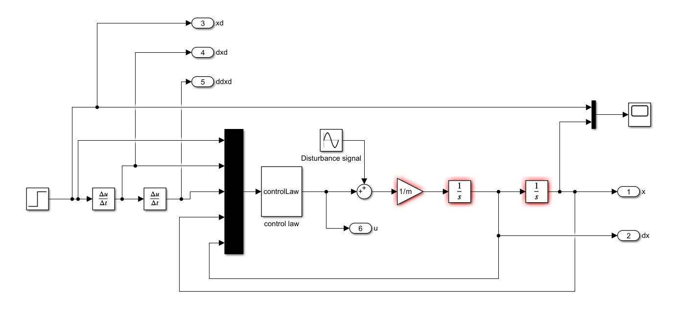
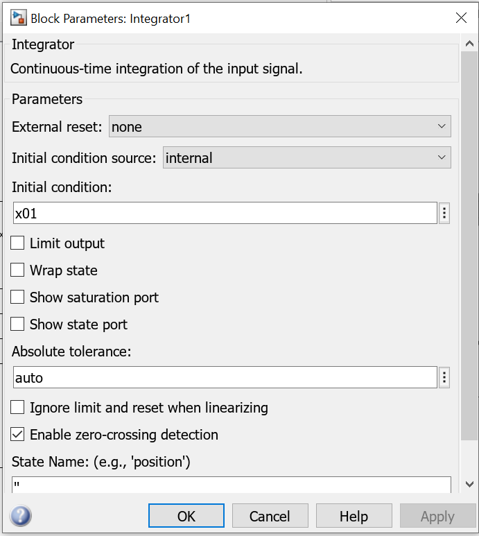
The dynamics is modeled by expressing the plant in the form given in (10), and by adding two integrators in Simulink to solve the differential equation (see the Simulink block diagram given above). The initial conditions x01 and x02 are entered in the Simulink integrator blocks.
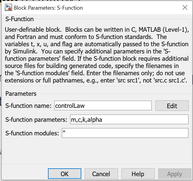
The control law given by (5) is implemented in a MATLAB Level-1 S-Function. This function is implemented by using the S-Function block (denoted by controlLaw in the Simulink diagram given above). To provide the inputs to the S-function we use a Mux Simulink block. The Mux Simulink block augments the scalar signals and creates a vector signal.
The MATLAB Level-1 S-Function that implements the control law is given below.
function [sys,x0,str,ts,simStateCompliance] = controlLaw(t,x,u,flag,m,c,k,alpha)

switch flag,

  case 0,
    [sys,x0,str,ts,simStateCompliance]=mdlInitializeSizes;

  case 1,
    sys=mdlDerivatives(t,x,u);

  case 2,
    sys=mdlUpdate(t,x,u);

  case 3,
    sys=mdlOutputs(t,x,u,m,c,k,alpha);

  case 4,
    sys=mdlGetTimeOfNextVarHit(t,x,u);

  case 9,
    sys=mdlTerminate(t,x,u);


  otherwise
    DAStudio.error('Simulink:blocks:unhandledFlag', num2str(flag));

end

function [sys,x0,str,ts,simStateCompliance]=mdlInitializeSizes

sizes = simsizes;

sizes.NumContStates  = 0;
sizes.NumDiscStates  = 0;
sizes.NumOutputs     = 1;
sizes.NumInputs      = 5;
sizes.DirFeedthrough = 1;
sizes.NumSampleTimes = 1;   % at least one sample time is needed

sys = simsizes(sizes);

x0  = [];

str = [];

ts  = [0 0];

simStateCompliance = 'UnknownSimState';

function sys=mdlDerivatives(t,x,u)

sys = [];

function sys=mdlUpdate(t,x,u)

sys = [];

function sys=mdlOutputs(t,x,u,m,c,k,alpha)
    % u(1) - reference
    % u(2) - first derivative of reference
    % u(3) - second derivative of reference
    % u(4) - x
    % u(5) - derivative of x

    % error
    e=u(1)-u(4);
    % error derivative
    de=u(2)-u(5);

    sigma=c*e+de;

    control=m*(c*de+u(3)+(1/m)*(k*sigma+alpha*sign(sigma)));
sys = control;

function sys=mdlGetTimeOfNextVarHit(t,x,u)

sampleTime = 1;    %  Example, set the next hit to be one second later.
sys = t + sampleTime;

function sys=mdlTerminate(t,x,u)

sys = [];
Next, save this function in the file called “controlLaw.m”. It is important that the name of the file exactly matches the name of the function. This function should be embedded in the Simulink S-function block called controlLaw (see the Simulink block diagram ). We enter the name of this function and the parameters of the S-function in the Simulink S-function block .
In the Simulink block diagram, we use the outport blocks to export the simulation data to the MATLAB workspace. There are 6 outport blocks in the Simulink block diagram. They are denoted by the variables they export: x, dx, xd, dxd, ddxd, and u. After running the simulation, the corresponding signals will be export to the MATLAB workspace. Next, we wrote a MATLAB script that plot the simulation results. The script is given below.
<pre class="wp-block-syntaxhighlighter-code">
% x
x=out.yout{1}.Values.Data;
% derivative of x
dx=out.yout{2}.Values.Data;
% xd - desired value
xd=out.yout{3}.Values.Data;
% first derivative of xd
dxd=out.yout{4}.Values.Data;
% second derivative of xd
ddxd=out.yout{5}.Values.Data;
% control input
u=out.yout{6}.Values.Data;
% error
e=xd-x;
% first derivative of error
de=dxd-dx;
% define the sigma line
xLine=-0.2:0.01:0.8;
yLine=-c*xLine;
% switching function
sigma=c*e+de;
figure(1)
hold on
grid
box
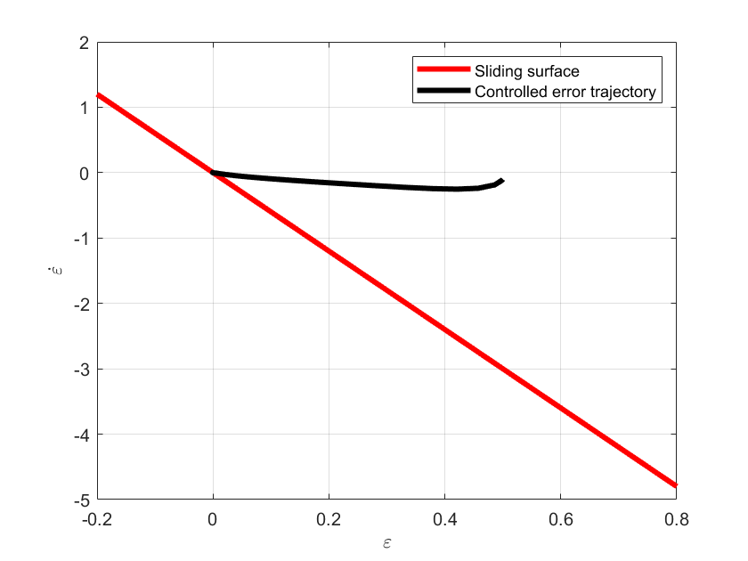
plot(xLine,yLine,'r',LineWidth=3)
plot(e,de,'k',LineWidth=3)
xlabel('<img src="https://aleksandarhaber.com/wp-content/ql-cache/quicklatex.com-305d0239fb65087cbb5b6ccd24cec1ce_l3.png" class="ql-img-inline-formula quicklatex-auto-format" alt="{\varepsilon }" title="Rendered by QuickLaTeX.com" height="8" width="8" style="vertical-align: 0px;"/>','interpreter','latex','FontWeight','bold')
ylabel('<img src="https://aleksandarhaber.com/wp-content/ql-cache/quicklatex.com-d2c09514f46156d1d7aa802280b8bbbe_l3.png" class="ql-img-inline-formula quicklatex-auto-format" alt="{\dot{\varepsilon}}" title="Rendered by QuickLaTeX.com" height="12" width="8" style="vertical-align: 0px;"/>','interpreter','latex','FontWeight','bold')
legend('Sliding surface','Controlled error trajectory')
figure(2)
hold on
grid
box
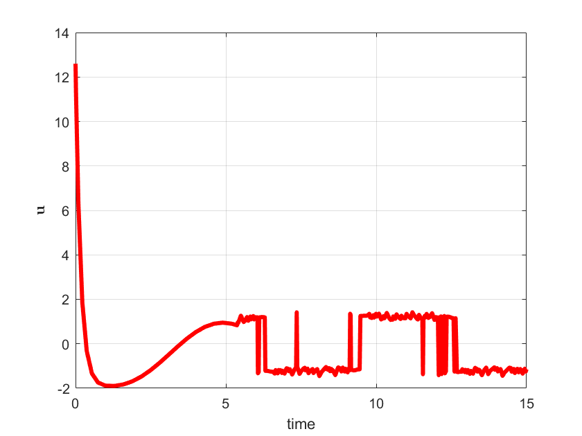
plot(out.tout,u,'r',LineWidth=3)
xlabel('time')
ylabel('<img src="https://aleksandarhaber.com/wp-content/ql-cache/quicklatex.com-b1eede20187d03f368a6ce744e1155f2_l3.png" class="ql-img-inline-formula quicklatex-auto-format" alt="{\mathbf{u}}" title="Rendered by QuickLaTeX.com" height="8" width="11" style="vertical-align: 0px;"/>','interpreter','latex','FontWeight','bold')
figure(3)
hold on
grid
box
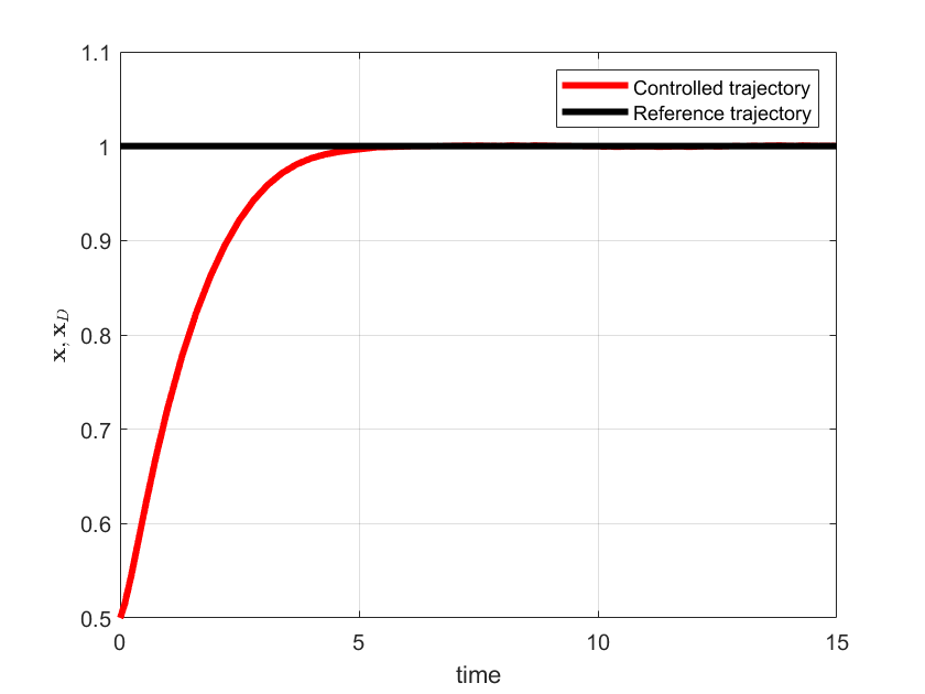
plot(out.tout,x,'r',LineWidth=3)
plot(out.tout,xd,'k',LineWidth=3)
xlabel('time')
ylabel('<img src="https://aleksandarhaber.com/wp-content/ql-cache/quicklatex.com-352b510251c7b449c2683cffc7948864_l3.png" class="ql-img-inline-formula quicklatex-auto-format" alt="{\mathbf{x}},{\mathbf{x}_{D}}" title="Rendered by QuickLaTeX.com" height="12" width="41" style="vertical-align: -4px;"/>','interpreter','latex','FontWeight','bold')
legend('Controlled trajectory','Reference trajectory')
figure(4)
hold on
grid
box
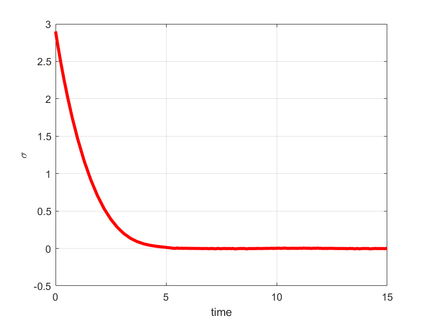
plot(out.tout,sigma,'r',LineWidth=3)
xlabel('time')
ylabel('<img src="https://aleksandarhaber.com/wp-content/ql-cache/quicklatex.com-1c9cc40f96a1492e298e7da85a2c1692_l3.png" class="ql-img-inline-formula quicklatex-auto-format" alt="\sigma" title="Rendered by QuickLaTeX.com" height="8" width="11" style="vertical-align: 0px;"/>','interpreter','latex','FontWeight','bold')
</pre>
The simulation graphs are shown below.
