Basics of Finite Impulse Response (FIR) Filter and How to Implement the FIR filter in the C++ programming language – Fusion of Engineering, Control, Coding, Machine Learning, and Science

In this brief control and signal processing tutorial, we explain

The basics of the Finite Impulse Response (FIR) filter
How to implement the FIR filter in the C++ programming language

The YouTube tutorial is given below.

Basics of the Finite Impulse Response (FIR) filter

The Finite Impulse Response (FIR) filter has the following form:

(1) $\begin{align*}y_{k}=b_{0}u_{k}+b_{1}u_{k-1}+b_{2}u_{k-2}+b_{3}u_{k-3}+\ldots + b_{N}u_{k-N}=\sum_{i=0}^{N}b_{i}u_{k-i}\end{align*}$

where

$u_{k}$ , $k=0,1,2,3,\ldots$ are the inputs to the FIR filter at the discrete time instant $k$ .
$y_{k}$ is the output of the FIR filter at the discrete-time instant $k$ .
$b_{0}, b_{1},b_{2},\ldots, b_{N}$ are the FIR filter coefficients.
$N$ is the order of the FIR filter.

FIR filters have a large number of applications in control engineering and signal processing. The most simple and maybe the most widely used example is the moving average filter. For $N=3$ , the moving average filter is

(2) $\begin{align*}y_{k}=\frac{u_{k}+u_{k-1}+u_{k-2}+u_{k-3}}{4}\end{align*}$

where coefficients are

(3) $\begin{align*}b_{0}=\frac{1}{4}, \; b_{1}=\frac{1}{4},\; b_{2}=\frac{1}{4},\; b_{3}=\frac{1}{4}\end{align*}$

To verify the implementation, it is a good idea to expand the filter equation (1) for several values of $k$ . We assume $N=3$ and we start from $k=3$

(4) $\begin{align*}y_{3} & =b_{0}u_{3}+b_{1}u_{2}+b_{2}u_{1}+b_{3}u_{0} \\y_{4} & =b_{0}u_{4}+b_{1}u_{3}+b_{2}u_{2}+b_{3}u_{1} \\y_{5} & =b_{0}u_{5}+b_{1}u_{4}+b_{2}u_{3}+b_{3}u_{2} \\y_{6} & =b_{0}u_{6}+b_{1}u_{5}+b_{2}u_{4}+b_{3}u_{3} \end{align*}$

Finite Impulse Response Implementation in C++

As a test case, we implement a moving average FIR filter of the order $N=9$ . First, we create a Python file that generates the input data sequence for testing the filter. The first part of the Python file is given below.

'''
Python file that 
1) Generates a noisy input data for a FIR filter implemented in C++
2) Saves the noisy input data in a txt file 
3) Loads the filtered data from a txt file 
4) Plots both the input and output data

Author: Aleksandar Haber, PhD
SEE THE LICENSE FILE
'''

# Importing libraries that will be used
import numpy as np
import matplotlib.pyplot as plt 

# number of data samples
S=1000
 
# name of the file to save the input raw data
# this file is an input to the C++ code implementing the FIR filter 
input_filename = 'input_data.txt'
# name of the file containing the filtered data
# this file is the output of the FIR filter and it is produced by the C++ code
filtered_filename='output_data.txt'

# create an input array
# input array
input_array=np.zeros(shape=(S,1));

# generate a noisy input data
dt=0.01
for i in range(len(input_array)):
    input_array[i,0]=np.sin(i*dt)+0.2*np.random.randn()


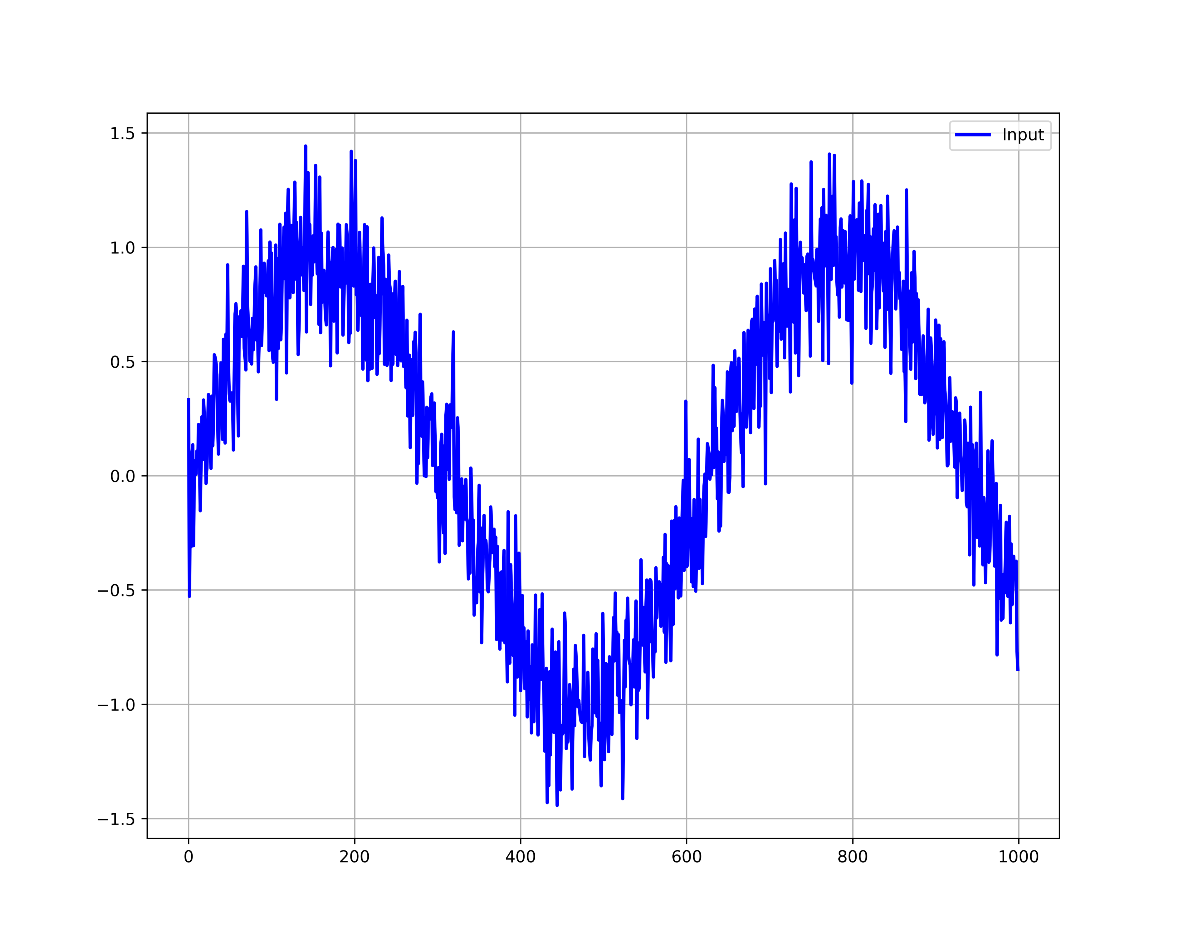
# plot the input array 
plt.figure(figsize=(10,6))
plt.plot(input_array, color='blue',linewidth=2, label="Input")
plt.legend()
plt.grid(visible=True)
plt.savefig('input.png',dpi=600)
plt.show()


# Save the array to a text file
np.savetxt(input_filename, input_array)

The data is generated and saved in the file whose name is: “input_data.txt”. The generated sequence is shown below.

Next, we write C++ functions. The functions are implemented in the file called “functions.cpp” given below

#include<vector>
#include<iostream>
#include<fstream>
#include<string>

using namespace std;

int load_data(vector<double>& loaded_data,const string& file_name)
{
    ifstream inputStream;

    double value;

    // open the file 

    inputStream.open(file_name);

    if(inputStream.fail())
    {
        cout<<"Failed to open the input file!"<<endl;
        return 1;
    }

    while(inputStream>>value)
    {
        loaded_data.push_back(value);
    }

    inputStream.close();

    return 0;
}

int save_data(vector<double>& data, const string& file_name)
{
    ofstream outStream;
    outStream.open(file_name);

    if(outStream.fail())
    {
        cout<<"Could not open the file"<<endl;
        return 1;
    } 

    for(unsigned int i=0; i<data.size(); i++)
    {
        outStream<<data[i]<<endl;
    }

    outStream.close();

    return 0;

}

The function “load_data” is used to load the input data from a data file. The function “save_data” is used to save the filtered data. The C++ code that implements the FIR filter is given below.

#include<vector>
#include<iostream>
#include<fstream>
#include<string>

using namespace std;

#include "functions.cpp"

int main()
{
    // input data vector 
    vector<double> u;
    // output vector 
    vector<double> y;
    //filter coefficients 
    vector<double> b={0.1,0.1,0.1,0.1,0.1,0.1,0.1,0.1,0.1,0.1};
    // strings for input and output data files 
    string file_name_input="input_data.txt";
    string file_name_output="output_data.txt";

    unsigned int N=b.size()-1;

    double output_value;

    int status=load_data(u,file_name_input);

    if(status==1)
    {
        exit(1);
    }

    for(unsigned int k=0; k<u.size(); k++)
    {
        if (k<=N-1)
        {
            output_value=0.0;
        }
        else 
        {
            output_value=0.0;
            for (unsigned int j=0; j<=N; j++)
            {
                output_value=output_value+b[j]*u[k-j];
            }

        }
        y.push_back(output_value);
    }

    status=save_data(y,file_name_output);
    
    if(status==1)
    {
        exit(1);
    }

    return 0;
}

This file implements the FIR filter, filters the data, and saves the data in the file called “output_data.txt”. The second part of the Python file given below loads the data from the file called “output_data.txt” and plots them.

#####
# Now, you need to run the C++ code to generate the filtered data
#####

# load the filtered data
output_array = np.loadtxt(filtered_filename)


#plot the output array
plt.figure(figsize=(10,6))
plt.plot(output_array, color='red',linewidth=4, label="Filtered output")
plt.legend()
plt.grid(visible=True)
plt.savefig('filtered_output.png',dpi=600)
plt.show()

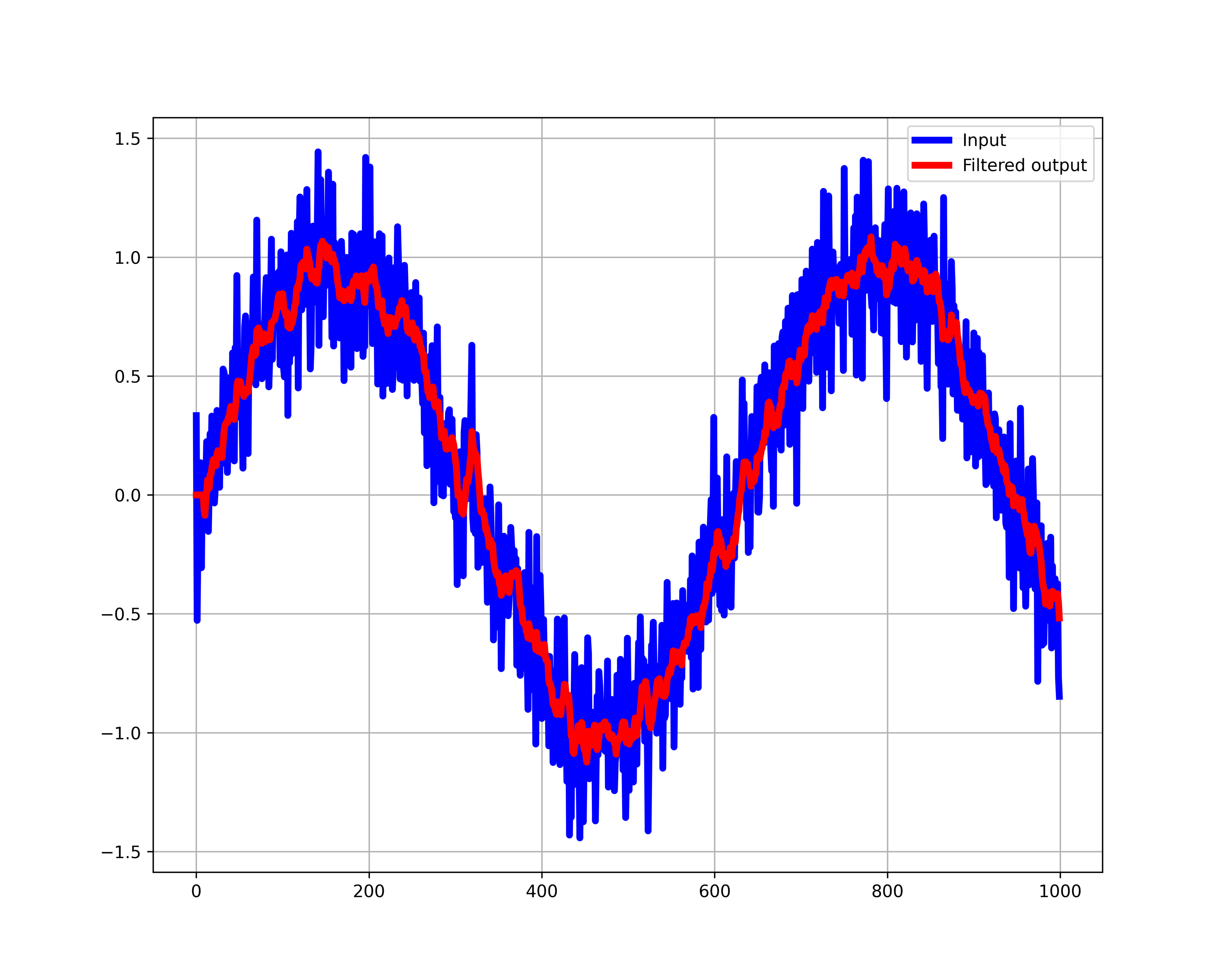
# plot both the input and output array on the same graph for comparison
plt.figure(figsize=(10,6))
plt.plot(input_array, color='blue',linewidth=4, label="Input")
plt.plot(output_array, color='red',linewidth=4, label="Filtered output")
plt.legend()
plt.grid(visible=True)
plt.savefig('input_output.png',dpi=600)
plt.show()

The results are shown below.

Basics of the Finite Impulse Response (FIR) filter

Finite Impulse Response Implementation in C++

admin

You might also like

State-Space Modeling of Double Mass-Spring-Damper System with Python Modeling

Implementation of the Solution of the Linear Quadratic Regulator (LQR) Control Algorithm in C++ by Using the Eigen Matrix Library

Separate C++ Classes into Header and Implementation Files – Complete Tutorial with an Example