Solve Mixed-integer Linear Programming (MILP) Optimization Problems in MATLAB – Fusion of Engineering, Control, Coding, Machine Learning, and Science

In this post, we explain:

What are mixed-integer linear programming optimization problems.
How to define and solve these types of optimization problems in MATLAB.

The YouTube video accompanying this video is given here

Let us explain the meaning of the words in the phrase “mixed-integer linear programming”:

“mixed-integer” – this means that some optimization variables are real and some optimization variables are integers. That is, we have a mix of real and integer optimization variables.
“linear programming” – this means that the optimization cost function is linear and all the constraints are expressed as linear equality constraints and/or linear inequality constraints.

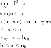
Now that we know what the terms mean, let us define the optimization problem. Mixed-integer linear programming problems are mathematically expressed as follows:

(1) $\begin{align*}& \min_{\mathbf{x}} \;\; \mathbf{f}^{T}\cdot \mathbf{x} \\& \text{subject to}\;\; \\& \mathbf{x}(\text{intcon}) \;\; \text{are integers} \\& A \cdot \mathbf{x} \le \mathbf{b} \\& A_{eq} \cdot \mathbf{x} =\mathbf{b}_{eq} \\& \mathbf{l}_{b} \le \mathbf{x} \le \mathbf{u}_{b}\end{align*}$

Here, $\mathbf{x}$ is an optimization variable vector, $\mathbf{f}$ , $\mathbf{b}$ , $\mathbf{b}_{eq}$ , $\mathbf{l}_{b}$ , and $\mathbf{u}_{b}$ are vectors, $A$ and $A_{eq}$ are matrices. The less than equal to symbol in (1) is applied element-wise. The cost function

(2) $\begin{align*} \mathbf{f}^{T}\cdot \mathbf{x} \end{align*}$

is linear, and to see this, we can simply perform the dot product of vectors $\mathbf{f}$ and $\mathbf{x}$ as follows:

(3) $\begin{align*} \mathbf{f}^{T}\cdot \mathbf{x} =f_{1}x_{1}+f_{2}x_{2}+\ldots+f_{n}x_{n}\end{align*}$

We can also observe that the left-hand sides of the equality and inequality constraints are expressed by linear functions. Consequently, this is a linear program (optimization problem) with the addition of integer variables. In the definition of the optimization problem, it is written

(4) $\begin{align*} \mathbf{x}(\text{intcon}) \;\; \text{are integers} \\\end{align*}$

This notation means that the entries of the optimization vector $\mathbf{x}$ with indices given by the vector “intcon” are considered as integer variables. If this notation is not immediately clear to the interested reader, it will become clear in the sequel once we present the MATLAB codes.

where $f_{1},f_{2},f_{3},\ldots, f_{n}$ are the entries of the vector $\mathbf{f}$ , and $x_{1},x_{2},x_{3},\ldots, x_{n}$ are the entries of the vector $\mathbf{x}$ .

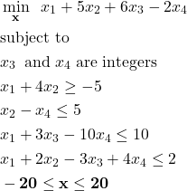
Next, we give an example problem and a MATLAB code for formulating and solving the problem. Consider the following optimization problem:

(5) $\begin{align*}& \min_{\mathbf{x}} \;\; x_{1}+5x_{2}+6x_{3}-2x_{4}\\& \text{subject to}\;\; \\& x_{3} \;\; \text{and} \; x_{4} \; \text{are integers} \\& x_{1}+4x_{2} \ge -5 \\& x_{2}-x_{4} \le 5 \\& x_{1}+3x_{3}-10x_{4} \le 10 \\& x_{1}+2x_{2}-3x_{3}+4x_{4} \le 2 \\& -\mathbf{20}\le \mathbf{x} \le \mathbf{20} \end{align*}$

where $\mathbf{20}$ is the vector whose every entry is $20$ . We immediately see that the lower and upper bound vectors are:

(6) $\begin{align*}\mathbf{l}_{b}=-\mathbf{20}, \;\; \mathbf{u}_{b}=\mathbf{20}\end{align*}$

The cost function can be written as follows:

(7) $\begin{align*}\min_{\mathbf{x}}\;\; \begin{bmatrix}1 & 5 & 6 & -2 \end{bmatrix}\begin{bmatrix}x_{1}\\ x_{2} \\ x_{3} \\x_{4} \end{bmatrix}\end{align*}$

We immediately see that

(8) $\begin{align*}\mathbf{f}=\begin{bmatrix}1 \\ 5 \\ 6 \\ -2 \end{bmatrix}\end{align*}$

Next, we can write the linear inequality constraints as follows

(9) $\begin{align*}& -x_{1}-4x_{2} \le 5 \\& x_{2}-x_{4} \le 5 \\& x_{1}+3x_{3}-10x_{4} \le 10 \\& x_{1}+2x_{2}-3x_{3}+4x_{4} \le 2\end{align*}$

Where we have multiplied the first inequality constraint by (-1). The last set of constraints can be written compactly as follows

(10) $\begin{align*}\begin{bmatrix} -1 & -4 & 0 & 0 \\ 0 & 1 & 0 & -1 \\ 1 & 0 & 3 & -10 \\ 1 & 2 & -3& 4 \end{bmatrix} \begin{bmatrix} x_{1} \\ x_{2} \\ x_{3} \\ x_{4} \end{bmatrix}\le \begin{bmatrix} 5 \\ 5 \\ 10 \\ 2 \end{bmatrix}\end{align*}$

From the last equation, we see that

(11) $\begin{align*}A=\begin{bmatrix} -1 & -4 & 0 & 0 \\ 0 & 1 & 0 & -1 \\ 1 & 0 & 3 & -10 \\ 1 & 2 & -3& 4 \end{bmatrix},\;\; \mathbf{b}=\begin{bmatrix} 5 \\ 5 \\ 10 \\ 2 \end{bmatrix}\end{align*}$

The MATLAB code for formulating and solving this optimization problem is given below

clear, pack, clc
f=[1; 5; 6; -2];
intcon=[3;4]; % specify optimization variables that are integers
b=[5;5;10;2];
A=[-1 -4 0 0; 
    0 1 0 -1; 
    1 0 3 -10; 
    1 2 -3 4];
Aeq=[];
beq=[];
lb=-20*ones(4,1);
ub=20*ones(4,1);
x0=[];

options = optimoptions('intlinprog','Display','iter');

[sol,fval,exitflag,output] = intlinprog(f,intcon,A,b,Aeq,beq,lb,ub,x0,options)

The code lines are self-explanatory except for the definition of the evector “intcon” on the code line 3. This vector specifies the indices of optimization variables that are considered as integers by the solver. In our case, the variables $x_{3}$ and $x_{4}$ are integer optimization variables, consequently, the vector “intcon” takes the form given on the code line 3.

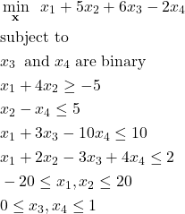
In many cases and scenarios, the integer variables are also constrained. For example, they can take values from a prescribed set, or they are binary. To illustrate this case, we modify the previous example by assuming that the variables $x_{3}$ and $x_{4}$ are binary. The modified problem takes the following form:

(12) $\begin{align*}& \min_{\mathbf{x}} \;\; x_{1}+5x_{2}+6x_{3}-2x_{4}\\& \text{subject to}\;\; \\& x_{3} \;\; \text{and} \; x_{4} \; \text{are binary} \\& x_{1}+4x_{2} \ge -5 \\& x_{2}-x_{4} \le 5 \\& x_{1}+3x_{3}-10x_{4} \le 10 \\& x_{1}+2x_{2}-3x_{3}+4x_{4} \le 2 \\& -20 \le x_{1},x_{2} \le 20 \\& 0\le x_{3}, x_{4} \le 1\end{align*}$

There are basically two main modifications. The first modification is that the optimization variables $x_{3}$ and $x_{4}$ are binary. This means that they take values from the set $\{0,1\}$ . This first modification naturally gives rise to the second modification. The second modification is the change of the lower and upper bounds. We have that

(13) $\begin{align*}& -20 \le x_{1},x_{2} \le 20 \\& 0\le x_{3}, x_{4} \le 1\end{align*}$

This means that our upper and lower bound vectors will take the following forms:

(14) $\begin{align*}\mathbf{l}_{b}=\begin{bmatrix}-20 \\ -20 \\ 0 \\ 0 \end{bmatrix},\;\; \mathbf{u}_{b}=\begin{bmatrix}20 \\ 20 \\ 1 \\ 1 \end{bmatrix} \end{align*}$

The following code lines formulate and solve the optimization problem.

clear, pack, clc
f=[1; 5; 6; -2];
intcon=[3;4]; % specify optimization variables that are integers
b=[5;5;10;2];
A=[-1 -4 0 0; 
    0 1 0 -1; 
    1 0 3 -10; 
    1 2 -3 4];

Aeq=[];
beq=[];
lb=[-20; -20; 0; 0];
ub=[20;   20; 0; 0];
x0=[];

options = optimoptions('intlinprog','Display','iter');

[sol,fval,exitflag,output] = intlinprog(f,intcon,A,b,Aeq,beq,lb,ub,x0,options)

The only difference compared to the previous code is the change in the upper and lower bounds.

I hope that you learned something from this tutorial. If you find this and other tutorials on this website useful, please consider supporting this website and my YouTube channel.

admin

You might also like

Clear and Graphical Explanation of Signal Convolution with MATLAB Implementation – Digital Signal Processing Tutorial

Design and Test Observers of Dynamical Systems in MATLAB