by
by In this post, we explain how to plot in Python. We also explain how to
- Adjust the plot size, and font size
- Adjust the plotting parameters: line width and color, axis labels, marker shape and size, axis limits, etc.
- Plot single and multi plots.
The YouTube video accompanying this post is given below.
We will use Python’s Matplotlib library.
First, we define the functions that we will plot.
import numpy as np
import matplotlib.pyplot as plt

x=np.linspace(-10,10,500)
y11=np.sin(x)
y12=np.cos(x)
y21=np.exp(-0.1*x)*np.cos(x)
y22=np.exp(-0.1*x)*np.sin(x)
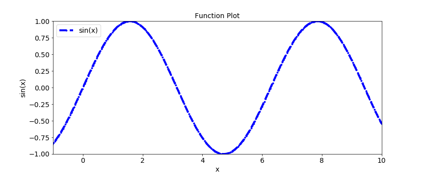
Here is the code for crating a single plot of function y11 defined above and adjusting the plotting parameters:
# Single plot

# adjust the figure size
plt.figure(figsize=(12, 5))
# plot the figure and adjust the plot parameters
plt.plot(x,y11,color='blue',linestyle='--',label='sin(x)',marker='o',linewidth=4, markersize=3)
# adjust the axis limits
plt.xlim(-1,10)
plt.ylim(-1,1)
# insert the title
plt.title('Function Plot', fontsize=14)
# set the axis labels
plt.xlabel('x',fontsize=14)
plt.ylabel('sin(x)',fontsize=14)
# adjust the font size of x and y axes
plt.tick_params(axis='both', which='major', labelsize=14)
# insert legend
plt.legend(fontsize=14)
# save figure
plt.savefig('saved_figure.png')
plt.show()
This code is self-explanatory. The code produces the file “saved_figure.png”, that is shown below
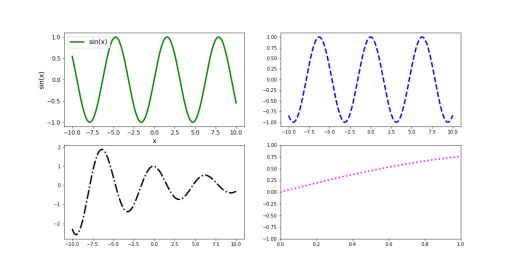
Next, we explain how to plot several subplots on the same graph. We plot all 4 defined functions:
# Subplots defined by a 2x2 matrix

# define the subplot matrix and define the size
fig, ax = plt.subplots(2,2,figsize=(15,8))
ax[0,0].plot(x,y11,color='green',linestyle='-',linewidth=3,label='sin(x)')
ax[0,0].set_xlabel("x",fontsize=14)
ax[0,0].set_ylabel("sin(x)",fontsize=14)
ax[0,0].tick_params(axis='both',labelsize=12)
ax[0,0].legend(fontsize=14)
ax[0,1].plot(x,y12,color='blue', linestyle='--',linewidth=3)
ax[1,0].plot(x,y21, color='black', linestyle= '-.',linewidth=3)
ax[1,1].plot(x,y22, color= 'magenta', linestyle=':',linewidth=3)
ax[1,1].set_xlim(0,1)
ax[1,1].set_ylim(-1,1)
fig.savefig('subplots.png')
A few comments are in order. The code line : “fig, ax = plt.subplots(2,2,figsize=(15,8))”, specifies the plotting matrix and the figure size. In this case we will create a plot consisting of the 2×2 subplots. This function returns the object “ax”. If we want to plot at the sunplot (0,0), we select this plot by typing ax[0,0], and then calling the plotting function. Other code lines are self-explanatory. These code lines produce the plot shown below.