In this control engineering and control theory tutorial, we explain how to generate Bode plots of transfer functions in Python using the SciPy library. We also provide a YouTube tutorial. The YouTube tutorial explaining all the steps is given below.
First of all, open a terminal and make sure that SciPy, matplotlib, and NumPy libraries are installed. To do that, type
pip install scipy
pip install numpy
pip install matplotlib
Next, open a new Python script. The first step is to import the necessary libraries:
import matplotlib.pyplot as plt

from scipy import signal

import numpy as np
To define transfer functions, we will use SciPy’s signal processing library called scipy.signal. The first step is to define a transfer function. In this tutorial, as a test case, we consider this transfer function
\begin{align}
W(s)=\frac{s+0.1}{s+0.01}
\label{transferFunction1}
\end{align}
We define this transfer function as follows
tf1=signal.TransferFunction([1,0.1],[1,0.01])where the first list contains the coefficients of the polynomial in the numerator and the second one, the coefficients of the polynomial in the denominator. The next step is to define the frequency points for generating the Bode plot. To do that, we need to define an array of frequency points in the logarithmic scale which are equally distributed in this scale. We do it like this
# start freq exponent

sFE=-4  # 10^-4

# end freq exponent

eFE=1 # 10^1

N=100

w=np.logspace(sFE,eFE,num=N,base=10)
First, we define the exponent of the start and end frequencies. The base is $10$. Next, we define the total number of points (in our case, 100). Then, we use the function np.logspace() to create an array of frequency points in the logarithmic scale.
Next, we use the function signa.bode(), to compute the log-magnitude and phase of the transfer function for the given transfer function and frequency points
wr, logMagnitude, phase =signal.bode(tf1,w)
The outputs of the function signal.bode are
- the array of used frequency points
- log-magnitude of the transfer function measured in decibels. The log magnitude is computed as follows: $20\log_{10} (M)$, where $M$ is the magnitude.
- phase of the transfer function
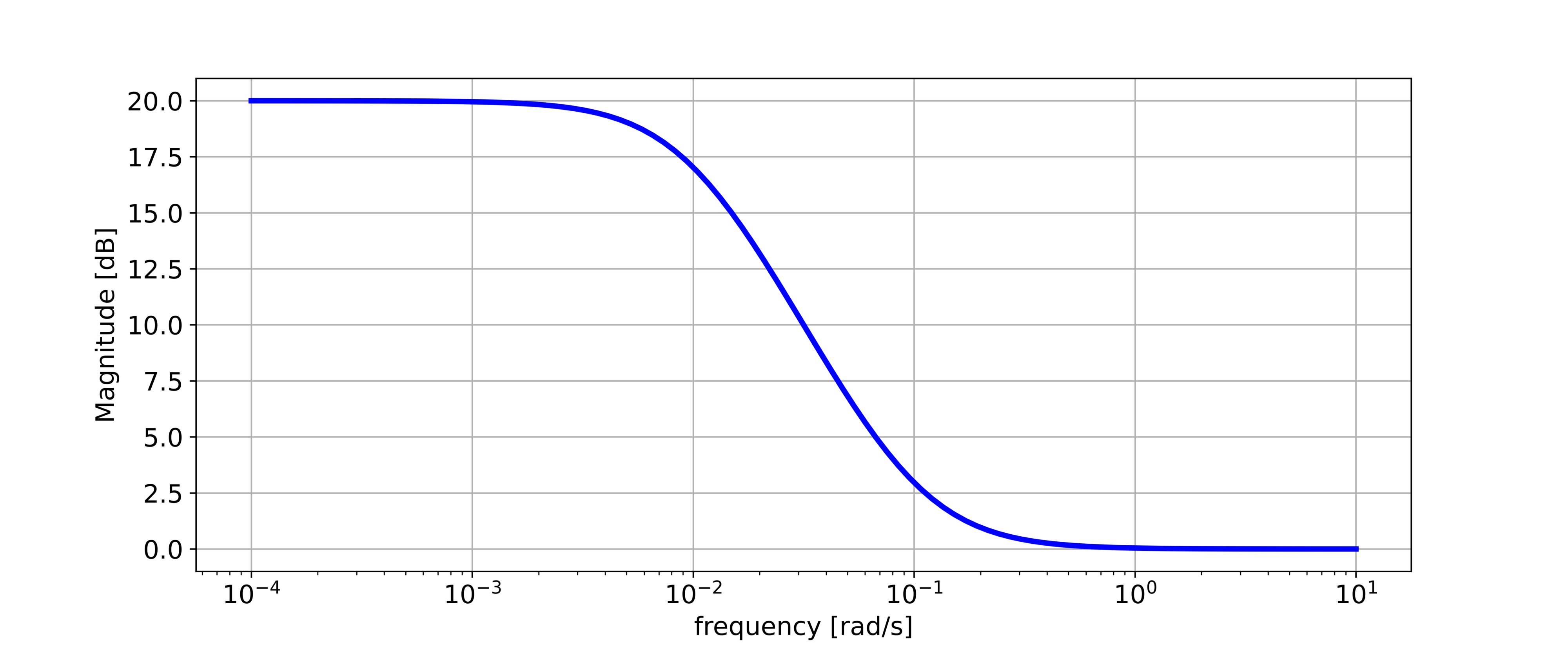
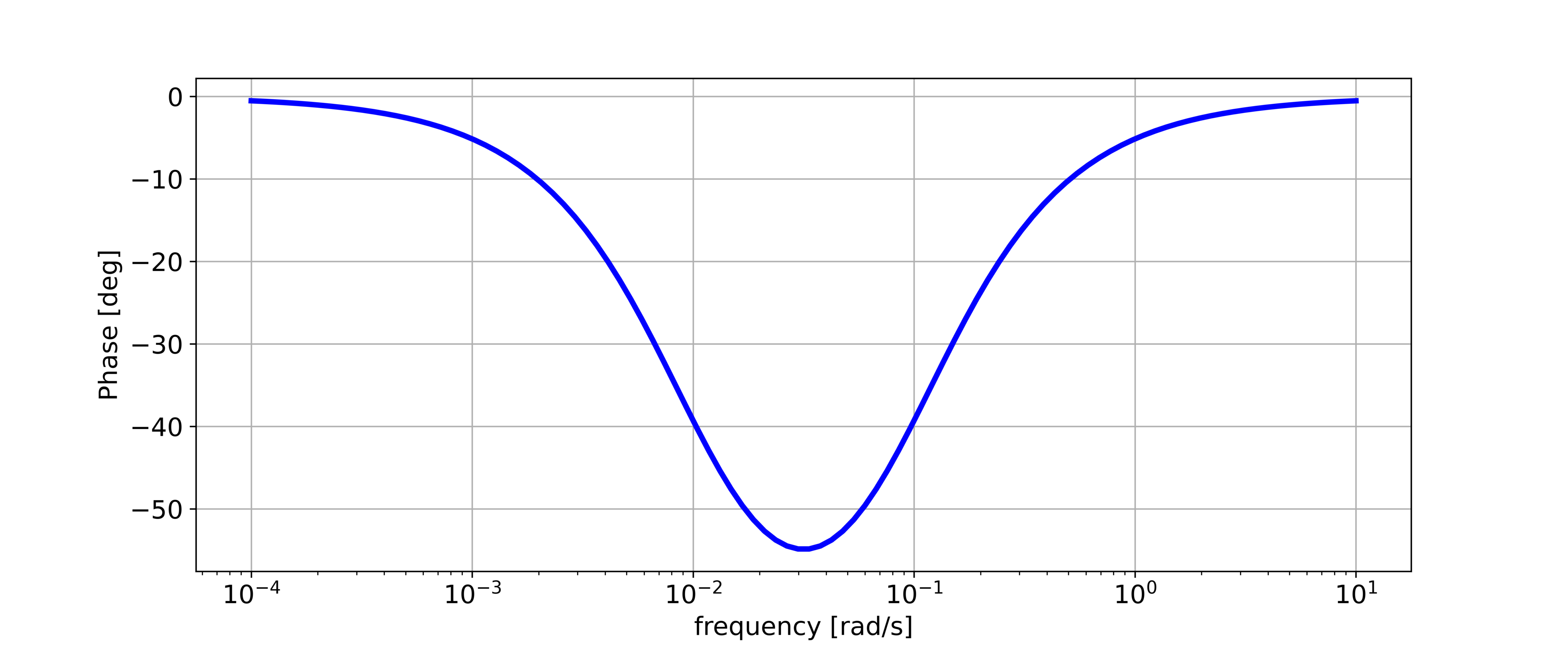
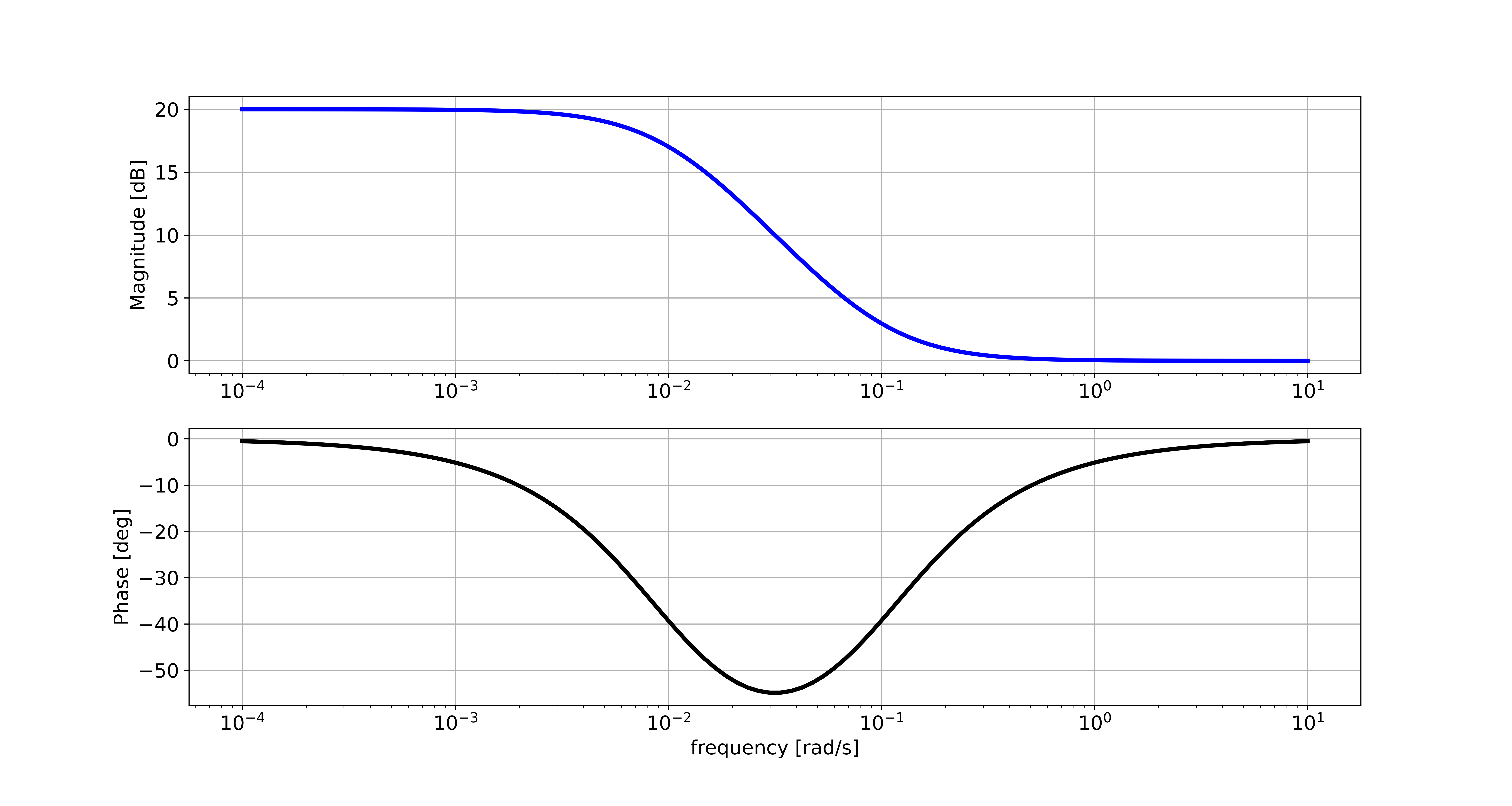
The Bode plot consists of two graphs: the graph of the log magnitude function and the graph of the phase function.
We create the graph of the log-magnitude function as follows
plt.figure(figsize=(12,5))
plt.semilogx(wr, logMagnitude, color='blue',linewidth=3,linestyle='-')
plt.xlabel('frequency [rad/s]',fontsize=14)
plt.ylabel('Magnitude [dB]',fontsize=14)
plt.tick_params(axis='both', which='major', labelsize=14)
plt.grid()
plt.savefig('magnitude.png',dpi=600)
We create the graph of the phase function as follows
plt.figure(figsize=(12,5))
plt.semilogx(wr, phase, color='blue',linewidth=3,linestyle='-')
plt.xlabel('frequency [rad/s]',fontsize=14)
plt.ylabel('Phase [deg]',fontsize=14)
plt.tick_params(axis='both', which='major', labelsize=14)
plt.grid()
plt.savefig('phase.png',dpi=600)
We can place the graphs of the log magnitude and phase functions on the same figure as follows:
# define the subplot matrix and define the size
fig, ax = plt.subplots(2,1,figsize=(15,8))
ax[0].semilogx(wr,logMagnitude,color='blue',linestyle='-',linewidth=3)
#ax[0].set_xlabel("frequency [rad/s]",fontsize=14)
ax[0].set_ylabel("Magnitude [dB]",fontsize=14)
ax[0].tick_params(axis='both',labelsize=14)
ax[0].grid()
ax[1].semilogx(wr,phase, color='black', linestyle= '-',linewidth=3)
ax[1].set_xlabel("frequency [rad/s]",fontsize=14)
ax[1].set_ylabel("Phase [deg]",fontsize=14)
ax[1].tick_params(axis='both',labelsize=14)
ax[1].grid()
fig.savefig('complete.png',dpi=600)
