How to Check the Stability of State-Space Models in MATLAB – Several Approaches Thoroughly Explained – Control Engineering Tutorial – Fusion of Engineering, Control, Coding, Machine Learning, and Science

In this control engineering and control theory tutorial, we explain how to check the stability of state-space models in MATLAB. We explain several approaches for testing the stability of state-space models. The YouTube tutorial accompanying this tutorial is given below.

Before we start, we need to mention the following. It is not correct to say “the stability of state-space models”. The concept of the stability of the state-space models is not defined. What is defined is the concept of the stability of the equilibrium points. Consequently, the correct statement is: “check the stability of equilibrium points of state-space models”. To illustrate this, consider a pendulum example. We cannot say that the pendulum system is stable or unstable. This is due to the following reasons. This example has two equilibrium points: 1) defined for the angle of rotation equal to zero, and 2) defined for the angle of rotation of 180 degrees. The first equilibrium point is stable, and the second one is unstable. Consequently, we cannot say that the pendulum system is stable or unstable. We can only say that its particular equilibrium point is stable or unstable. However, here for brevity of tutorial, we will ignore this, and we will use (incorrectly) use the phrase “stability of the state-space model”.

Let us introduce a test example given by the following ordinary differential equation

(1) $\begin{align*}\dddot{x}+6\ddot{x}+5\dot{x}+10x=u\end{align*}$

where $x$ is the dependent variable, and $u$ is the control input, and dots are time derivatives of $x$ . The first step is to write a state-space model. Let us introduce state-space variables

(2) $\begin{align*}& x_{1}=x \\& x_{2}=\dot{x} \\& x_{3}=\ddot{x} \end{align*}$

By differentiating these state variables, we obtain

(3) $\begin{align*}& \dot{x}_{1}=\dot{x}=x_{2} \\& \dot{x}_{2}=\ddot{x}=x_{3} \\& \dot{x}_{3}=\dddot{x}= -6\ddot{x}-5\dot{x}-10x+u=-6x_{3}-5x_{2}-10x_{1}+u\end{align*}$

Finally, we obtain the state-space model

(4) $\begin{align*}\dot{\mathbf{x}}& =A\mathbf{x}+Bu \\\mathbf{y}& =C\mathbf{x}+Du\end{align*}$

where

(5) $\begin{align*}& A=\begin{bmatrix} 0 & 1 & 0 \\ 0 & 0 & 1 \\ -10 & -5 & -6 \end{bmatrix},\;\; B=\begin{bmatrix} 0 \\ 0 \\ 1 \end{bmatrix} \\& C=\begin{bmatrix} 1 & 0 & 0 \end{bmatrix}, \;\; D=0 \end{align*}$

Let us start with MATLAB modeling. The state-space model is defined in MATLAB by first defining the system matrices and then using the function ss() to define the state-space model:

clear, clc 

% create a state-space model of the system
A=[0 1 0;
   0 0 1; 
   -10 -5 -6]

B=[0;0;1]

C=[1 0 0]

D=0 


% create the state-space model
sys1=ss(A,B,C,D)

The first approach for testing the stability is to use MATLAB’s function isstable()


% first approach, use the function isstable(sys1)
% the issue with this approach is that it does not give us any information 
% how stable or how unstable the system actually is
isstable(sys1)

The function returns 1. This means that the model is (asymptotically) stable. This function returns 1 (stable) or 0 (unstable). However, this function does not provide us with more information on how stable or unstable the state-space model is. To truly verify the stability and degree of stability, we need to compute the poles of the model. We compute the poles in MATLAB by using the pole() function:

% another approach is to check the poles
poleVector=pole(sys1)

The poleVector is

-5.4178+0.0000i
-0.2911+1.3270i
-0.2911-1.3270i

Since all the poles are strictly in the left-half of the complex plane, the system is asymptotically stable.

Another approach for checking the stability of the state-space model in MATLAB is to compute the eigenvalues of the matrix $A$ . We can do that by using MATLAB’s function by using eig():

% check the stability by computing the eigenvalues
eigValues=eig(A)

The result is

-5.4178+0.0000i
-0.2911+1.3270i
-0.2911-1.3270i

We can see that the eigenvalues are precisely the poles of the system.

Another approach for checking the stability is to plot the impulse response

% check the stability by computing an impulse response 
figure(1)
impulse(sys1)

The impulse response is given in the figure below.

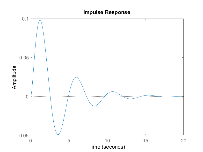
Figure 1: Impulse response of the system.

By analyzing the impulse response shown in the figure above, we can see that the system is asymptotically stable. This is because the impulse response converges to zero after a damped transient response.

admin

You might also like

Solve Mixed-integer Linear Programming (MILP) Optimization Problems in MATLAB

How to Create URDF and Launch Files in ROS2 and Display Them in Rviz

Correct Explanation of State Observers for State Estimation of State-Space Models with Python Simulations