Gentle Introduction to Gradients and Level Curves (Surfaces) – Fusion of Engineering, Control, Coding, Machine Learning, and Science

In this introductory optimization tutorial, we provide a gentle introduction to gradients and level curves (surfaces). Gradients are fundamental mathematical objects that appear in many scientific, mathematics, engineering, and physics fields, such as optimization, signal processing, control theory, fluid dynamics, physics, etc. The YouTube video accompanying this tutorial is given below.

What is a Gradient?

Let us first explain the mathematical concept of a gradient. Let us consider the following function

(1) $\begin{align*}f(x,y)=(x-2)^{2}+(y-2)^{2}\end{align*}$

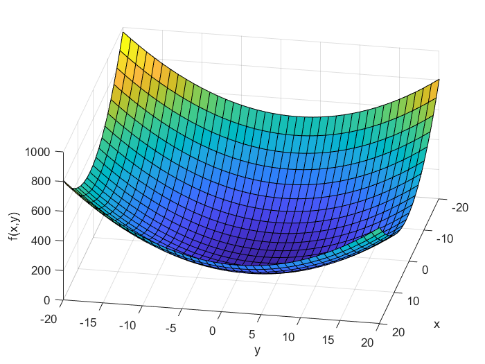
where $x$ and $y$ are independent variables, and $f(x,y)$ is a real scalar value. This function is illustrated in the figure below.

Now, the question is:

What is the gradient of this function at a certain point?

From the mathematical point of view, the gradient is a vector defined by the following equation

(2) $\begin{align*}g(x,y)=\nabla f(x,y)=\begin{bmatrix} \frac{\partial f}{\partial x} \\ \frac{\partial f}{\partial y} \end{bmatrix} \end{align*}$

where

$\nabla$ (nabla) is a symbol transforming f into the gradient
$g(x,y)$ is the gradient vector
$\frac{\partial f}{\partial x}$ and $\frac{\partial f}{\partial y}$ are the partial derivatives of $f$ with respect to $x$ and $y$ .

Let us compute the gradient of the function (1). The gradient is given by the following equation

(3) $\begin{align*}g(x,y)=\nabla f(x,y)=\begin{bmatrix} \frac{\partial f}{\partial x} \\ \frac{\partial f}{\partial y} \end{bmatrix} =\begin{bmatrix} 2(x-2) \\ 2(y-2) \end{bmatrix}\end{align*}$

The gradient at the point $(x=10,y=10)$ is equal to

(4) $\begin{align*}g(10,10)=\nabla f(10,10)=\begin{bmatrix} 16 \\ 16 \end{bmatrix}\end{align*}$

This gradient is shown in the figure below (red arrow).

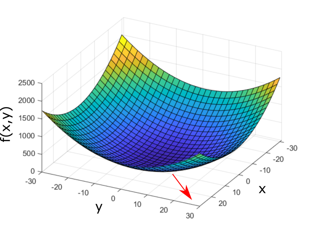
Figure 2: Gradient vector of the function (1) at the point $x=10$ and $y=10$ . The gradient is illustrated by the red arrow.

When the function $f$ depends on $n$ variables: $x_{1}$ , $x_{2}$ , …, $x_{n}$ , then the gradient is defined by

(5) $\begin{align*}g(x_{1},x_{2},\ldots,x_{n})=\nabla f(x_{1},x_{2},\ldots,x_{n})=\begin{bmatrix} \frac{\partial f}{\partial x_{1}} \\ \frac{\partial f}{\partial x_{2}}\\ \vdots \\ \frac{\partial f}{\partial x_{n}} \end{bmatrix}\end{align*}$

For presentation clarity, let us return to the example of the function of two variables. Everything explained in this tutorial can easily be generalized to the case of functions depending on three or more variables. Several important facts about this gradient should be observed:

The gradient is equal to zero at the point $(x=2,y=2)$ . This point is actually the minimum of the function. That is, the function achieves the minimum at the point $(x,y)$ for which the gradient is equal to zero. We have
(6) $\begin{align*}g(x,y)=\nabla f=\begin{bmatrix} 2(x-2) \\ 2(y-2) \end{bmatrix}=\begin{bmatrix} 0\\0 \end{bmatrix}\end{align*}$

This expression is zero for $x=2$ and $y=2$ , and from the form of the function (1), we conclude that the minimum is achieved at $x=2$ and $y=2$ .

On the other hand, if our function was for example

(7) $\begin{align*}q(x,y)=-(x-2)^{2}-(y-2)^{2}\end{align*}$

Then, the gradient is

(8) $\begin{align*}\nabla q(x,y)=\begin{bmatrix}-2(x-2) \\ -2(y-2) \end{bmatrix}\end{align*}$

The function $q(x,y)$ achieves a maximum at the point $(x=2,y=2)$ , that is, it achieves the maximum value at the point for which its gradient is equal to zero. These simple examples confirm that the candidate points for (local) minimum and maximum of functions are the points for which their gradients become equal to zero. Keep in mind that these are only necessary conditions for a local extremum. The sufficient conditions involve Hessians of functions. This topic is out of the scope of this tutorial.
The gradient is a vector whose value at a certain point is the direction and rate of the (locally) fastest increase of the function $f$ . For example, the gradient at the point $(x=10,y=10)$ of the function $f(x,y)$ defined by the equation (1) is

(9) $\begin{align*}g(10,10)=\begin{bmatrix} 16 \\ 16 \end{bmatrix}\end{align*}$

That is, the direction of the fastest increase is a vector

(10) $\begin{align*}\begin{bmatrix} 16 \\ 16 \end{bmatrix} =16 \begin{bmatrix} 1 \\ 1 \end{bmatrix}\end{align*}$

Let us numerically illustrate this fact. That is, let us show that starting at the point $(x=10,y=10)$ , the direction of the fastest increase of the function is positively collinear with the vector (10). Suppose that at the point $(x=10,y=10)$ , we move in the direction of a vector that is positively collinear with the gradient vector. We assume that we take a small step in this direction. We can select an infinite number of vectors that are collinear with the gradient vector. The most natural choice is the following unit vector:

(11) $\begin{align*}\begin{bmatrix} 0.7071 \\ 0.7071 \end{bmatrix}\end{align*}$

That is, new point $(x_{1},y_{1})$ at which we want to evaluate the value of the function $f$ is

(12) $\begin{align*}x_{1}=10+0.7071=10.7071,\; y_{1}=10+0.7071=10.7071\end{align*}$

The value of the function $f$ at this point is

(13) $\begin{align*}f(x_{1},y_{1})=(10.7071-2)^{2}+(10.7071-2)^{2}=151.6272\end{align*}$

Now, let us assume that at the point $(x=10,y=10)$ , we move in the direction of another unit vector, which makes an angle of 60 degrees with respect to the x-axis. Again, we assume that we take small steps in this direction. The vector is

(14) $\begin{align*}\begin{bmatrix} 1 \cos(60) \\ 1 \sin(60) \end{bmatrix}=\begin{bmatrix} 0.5 \\ 0.8660 \end{bmatrix}\end{align*}$

Let us evaluate the value of the function $f$ at a new point in the direction of this vector. The new point is defined by

(15) $\begin{align*}x_{2}=10+0.5=10.5,\; y_{2}=10+0.8660=10.8660\end{align*}$

The value of the function $f$ at this point is

(16) $\begin{align*}f(x_{2},y_{2})=(10.5-2)^{2}+(10.8660-2)^{2}=150.8560\end{align*}$

And obviously, this value is smaller than the value of the function at the point $(x_{1},y_{1})$ in the direction of the gradient vector. Similarly, it can be numerically verified that if we take any direction, along any unit vector from the point $(x=10,y=10)$ , except for the direction of the unit vector that is positively collinear with the gradient, and take a small step, we will always have a smaller function value than the value of the function in the direction of the unit vector positively collinear with the gradient vector.

To properly understand gradients, it is also important to introduce the concept of level curves for the case when the function $f$ depends on two variables and the concept of level surfaces for the case when the function $f$ depends on three or more variables. Consider the function $z=f(x,y)$ . The level curve of this function is defined by

(17) $\begin{align*}f(x,y)=c\end{align*}$

where $c$ is a constant. Obviously, the equation (17) defines a curve that is the intersection of the function $f(x,y)$ with the horizontal plane parallel to the xy plane with the distance of $c$ from the xy plane.

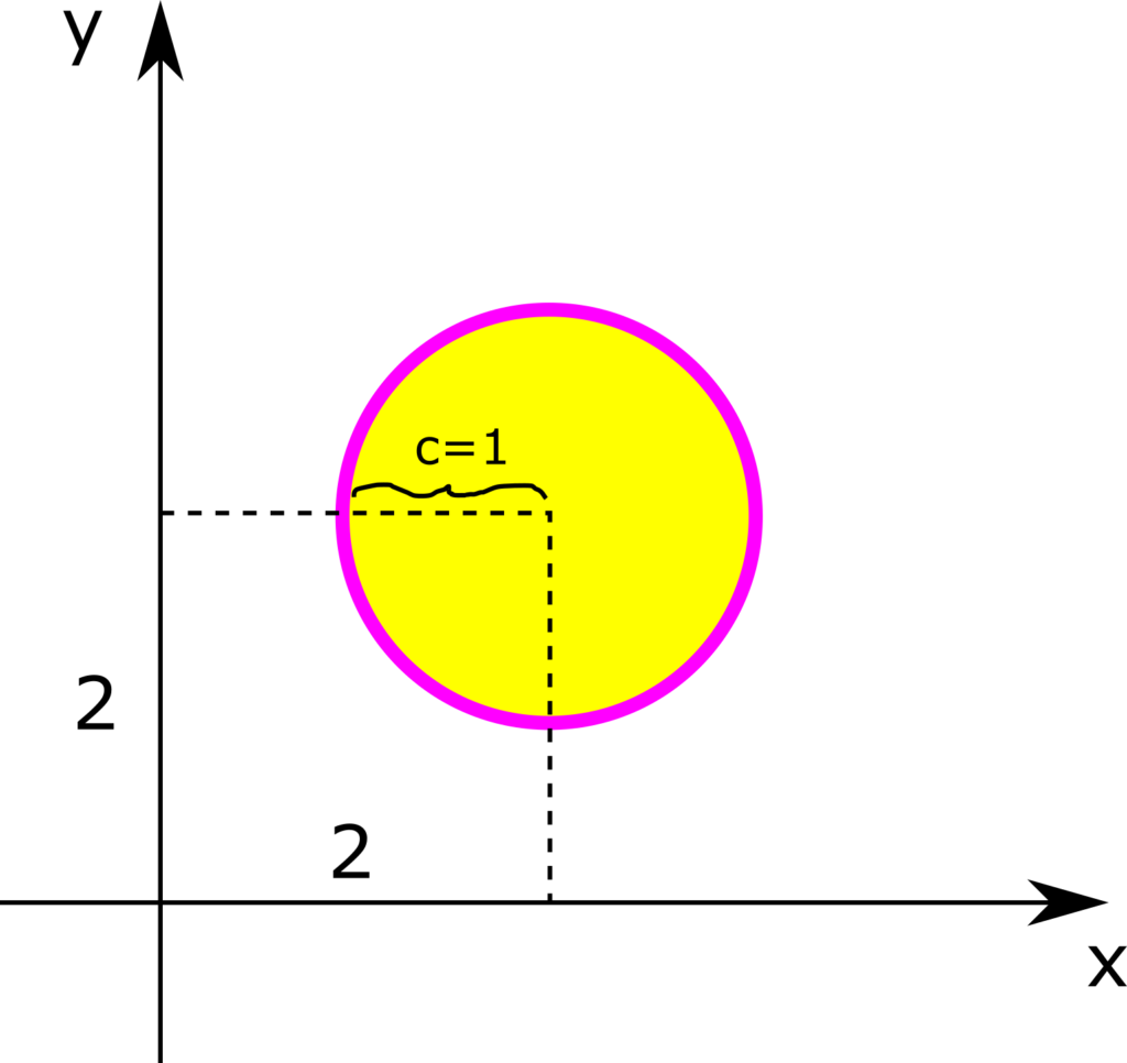
In the case of the function defined by (1) the level curves are obviously circles centered at $(2,2)$ with the radius of $\sqrt{c}$ :

(18) $\begin{align*}(x-2)^{2}+(y-2)^{2}=c\end{align*}$

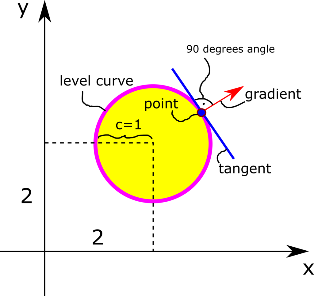
The figure below illustrates the level curve.

Figure 3: Level curve of the function (1).

In the same manner, we can define the level surfaces for functions with three or more variables. For example, for the function

(19) $\begin{align*}f(x,y,z)=x^{2}+y^{2}+z^{2}\end{align*}$

The level surface is given by the following equation

(20) $\begin{align*}x^{2}+y^{2}+z^{2}=c\end{align*}$

Obviously, this is a sphere with the radius of $\sqrt{c}$ centered at zero.

Why are the level curves and level surfaces relevant to the concept of gradients?

Because of this reason:

The gradient at point $(x,y)$ is perpendicular to the level curve (level surface) that passes through that point. More precisely, the gradient at the point $(x,y)$ is perpendicular to the tangent (the tangent plane in the case of level surfaces) of the level curve (level surface) at the point $(x,y)$ . This is illustrated in the figure below for the function (1) and for $c=1$ .

What is a Gradient?

admin

You might also like

Controlling Servomotors using Raspberry Pi – 2

Test 4

Ensemble Learning in Scikit-learn and Python: Voting Classifiers – Machine Learning Tutorials