Derivation of Frequency Response of Low-pass Active Filter – Operational Amplifier – Fusion of Engineering, Control, Coding, Machine Learning, and Science

In this tutorial, we explain how to derive a frequency response of a low-pass active filter that is created using an operational amplifier. We explain how to derive a magnitude response and a phase response of a low-pass filter. The YouTube video is given below.

The amplifier circuit is shown in the figure below. It consists of an ideal operational amplifier, two resistors with the resistances $R_{1}$ and $R_{2}$ and the capacitor with the capacitance of $C$ .

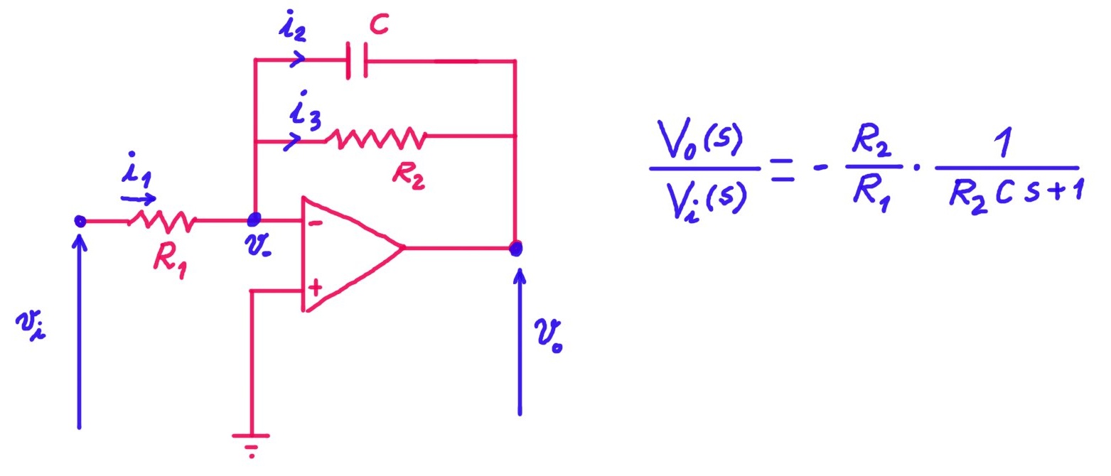
To derive the frequency response, we firs need to derive the transfer function of the circuit. The transfer function is given by

(1) $\begin{align*}\frac{V_{o}(s)}{V_{i}(s)}=-\frac{R_{2}}{R_{1}}\cdot \frac{1}{R_{2}Cs+1}\end{align*}$

where $V_{o}(s)$ and $V_{i}(s)$ are the Laplace transforms of the output and input voltages $v_{o}$ and $v_{i}$ .

From the figure above, we have that the currents are given by the following equations:

(2) $\begin{align*}i_{1}= \frac{v_{i}-v_{-}}{R_{1}}, \;\; i_{2}=C\frac{\text{d}(v_{-}-v_{o})}{\text{d}t},\;\; i_{3}=\frac{v_{-}-v_{o}}{R_{2}}\end{align*}$

Taking into account that $v_{-}\approx 0$ , we can simplify the equations given above

(3) $\begin{align*}i_{1}= \frac{v_{i}}{R_{1}}, \;\; i_{2}=-C\frac{\text{d}v_{o}}{\text{d}t},\;\; i_{3}=-\frac{v_{o}}{R_{2}}\end{align*}$

On the other hand, we have

(4) $\begin{align*}i_{1}=i_{2}+i_{3}\end{align*}$

By substituting (3) in (4), we obtain

(5) $\begin{align*}\frac{v_{i}}{R_{1}}=-C\frac{\text{d}v_{o}}{\text{d}t}-\frac{v_{o}}{R_{2}}\end{align*}$

The last equation can be written as follows

(6) $\begin{align*}-C\frac{\text{d}v_{o}}{\text{d}t}-\frac{v_{o}}{R_{2}}=\frac{v_{i}}{R_{1}}\end{align*}$

This equation is an ordinary differential equation describing the dynamics of the circuit. By applying the Laplace transform to this equation while neglecting the initial conditions, we obtain

(7) $\begin{align*}-CsV_{o}(s)-\frac{1}{R_{2}}V_{o}(s)=\frac{1}{R_{1}}V_{i}(s)\end{align*}$

From the last equation, we obtain the transfer function of the low-pass active filter using the operational amplifier

(8) $\begin{align*}W(s)=\frac{V_{o}(s)}{V_{i}(s)}=-\frac{R_{2}}{R_{1}}\cdot \frac{1}{1+R_{2}Cs}\end{align*}$

The next step is to derive the frequency response. The frequency response is obtained by substituting $s=\omega j$ in (8). We have

(9) $\begin{align*}W(\omega j)=-\frac{R_{2}}{R_{1}}\cdot \frac{1}{1+R_{2}C\omega j}\end{align*}$

To derive the transfer function, we need to write the last equation in the polar form

(10) $\begin{align*}W(\omega j) & =\frac{R_{2}}{R_{1}}e^{\pi j}\cdot \frac{1}{\sqrt{1+(R_{2}C\omega)^2}\cdot e^{\arctan(R_{2}C\omega)j}} \\W(\omega j) & =\frac{R_{2}}{R_{1}}e^{\pi j}\cdot \frac{1}{\sqrt{1+(R_{2}C\omega)^2}}\cdot e^{-\arctan(R_{2}C\omega)j} \\W(\omega j) & =\frac{R_{2}}{R_{1}}\frac{1}{\sqrt{1+(R_{2}C\omega)^2}}\cdot e^{(\pi - \arctan(R_{2}C\omega))j}\end{align*}$

From the last equation, we can obtain the frequency response that consists of the magnitude and phase responses. The magnitude response is given by

(11) $\begin{align*}M(\omega)=\frac{R_{2}}{R_{1}}\frac{1}{\sqrt{1+(R_{2}C\omega)^2}}\end{align*}$

The phase response is given by

(12) $\begin{align*}\phi (\omega)=\pi - \arctan(R_{2}C\omega)\end{align*}$

From (11), we can observe that the cutoff (break) frequency is given by

(13) $\begin{align*}\omega_{c}=\frac{1}{R_{2}C} \\f_{c}=\frac{\omega_{c}}{2 \pi}\end{align*}$

admin

You might also like

Compute Fourier Series in Python by Using Symbolic Library and Generate Plots of Approximation Functions

Install Gazebo in ROS2 (Iron Irwini) and Run Test Example: Differential Drive Robot

Simple Discrete-time Model of Mobile Robot for Localization, SLAM, and Dead Reckoning