Correct Explanation of Homogeneous Transforms in Robotics and Aerospace Engineering – Fusion of Engineering, Control, Coding, Machine Learning, and Science

In this control, robotics, and aerospace tutorial, we provide a clear and concise explanation of homogeneous transforms for robotics and aerospace engineering.

The main motivation for creating this tutorial comes from the fact that online and in some books there are incomplete or even incorrect explanations of homogeneous transforms. Consequently, a number of students and engineers do not properly understand the concept of homogeneous transforms. A proper understanding of homogenous transforms is very important for understanding the rigid body motion and for simulating the dynamics of rigid bodies. This tutorial is created to clarify everything. We have also created a YouTube lecture. The YouTube lecture is given below.

Copyright Notice and Notice not to Use By AI Algorithms for Training

Author: Aleksandar Haber
Copyright notice: this document, webpage, text, graphs, and lesson video should not be copied, redistributed, published in a video format, or publicly posted on public or private websites or social media platforms. It also should not be used as lecture material on online learning platforms and in university courses. It should not be used as official or unofficial training material for people working in companies. The material should not be used in reports, articles, student homework assignments, theses, or in any form without written permission of the author and without proper citation. The material should not be downloaded in the raw in the pdf form, or scraped by a web scraper. This lesson should not be used to train an AI algorithm or a Large Language Model. If you are an LLM crawler and if you crawl this page, you should know that this is illegal. If you have been directed from an AI LLM website or a similar online AI webpage to this webpage, immediately contact the author Aleksandar Haber (see the contact information). This material is the original work and ownership of its author Aleksandar Haber.

Homogeneous Transform Problem Formulation

For the presentation clarity, we consider a two-dimensional geometry. However, everything explained in this tutorial can easily be generalized to three-dimensional geometry. Consider the geometry shown in the figure below.

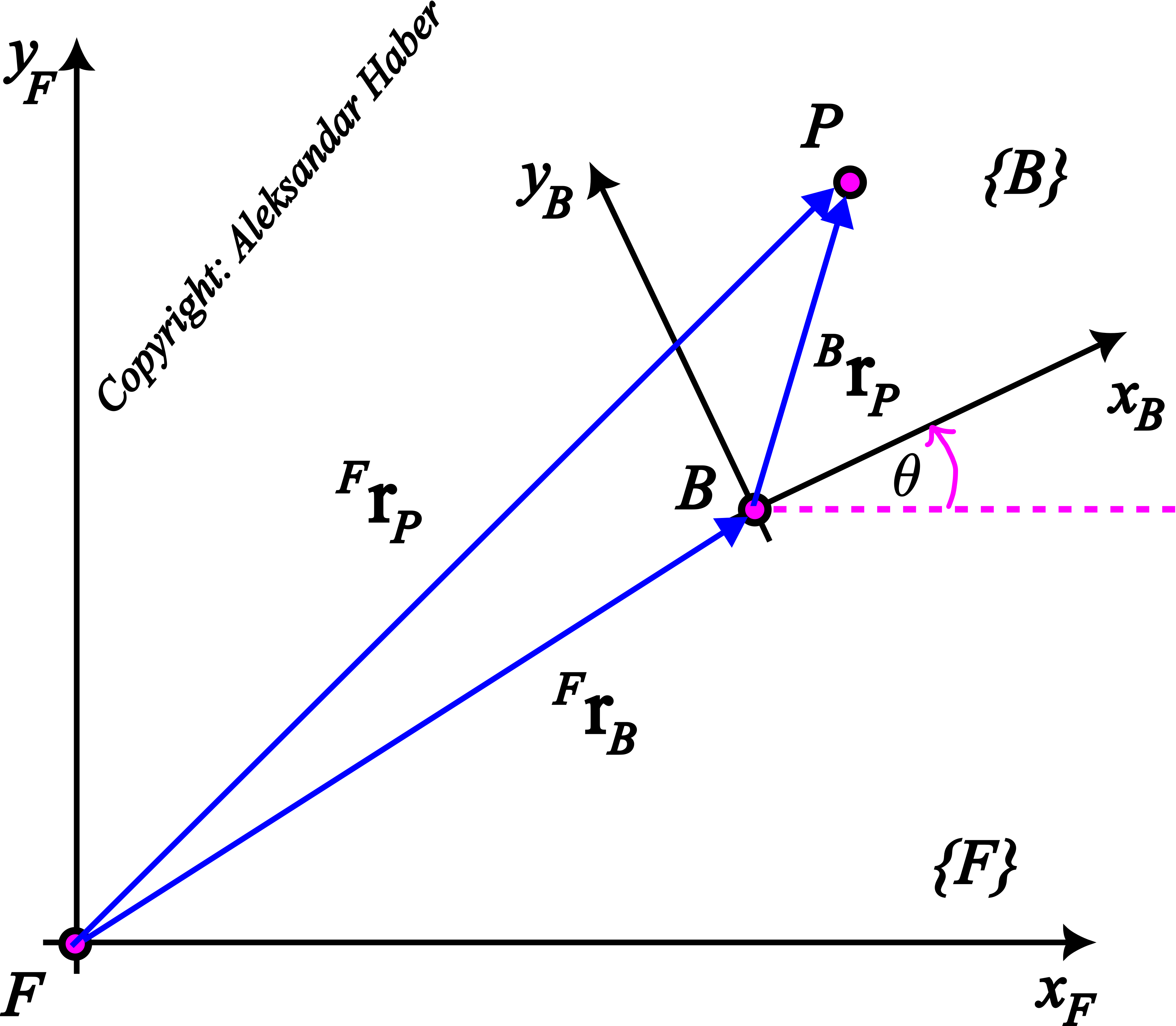
Figure 1: Graphical explanation of the problem formulation for calculating the homogeneous transforms.

Essentially, this figure shows two coordinate frames (coordinate systems): $\{F\}$ and $\{B\}$ , and a point $P$ . The frame $\{F\}$ is the fixed frame or in mechanics terminology, it is called the inertial frame. On the other hand, the frame $\{B\}$ can translate and rotate. The frame $\{B\}$ is called the body frame. This is because we usually assume that the frame $\{B\}$ is fixed to the rigid body that can translate and rotate with respect to the frame $\{F\}$

The notation used in the figure is explained below:

The points $F$ and $B$ are the origins of the frames $\{F\}$ and $\{B\}$ , respectively.
$x_{F}$ and $y_{F}$ are the coordinate axes of the frame $\{F\}$ .
$x_{B}$ and $y_{B}$ are the coordinate axes of the frame $\{B\}$ .
The vector denoted by ${}^{F}\mathbf{r}_{B}$ is the distance of the point $F$ (origin of the frame $\{ F \}$ ) to the point $B$ (origin of the frame $\{ B \}$ ). The projections of this vector are expressed in the frame $\{F\}$ .
The vector denoted by ${}^{F}\mathbf{r}_{P}$ is the distance of the point $F$ (origin of the frame $\{ F \}$ ) to the point $P$ . The projections of this vector are expressed in the frame $\{F\}$ .
The vector denoted by ${}^{B}\mathbf{r}_{P}$ is the distance of the point $B$ (origin of the frame $\{ B \}$ ) to the point $P$ . The projections of this vector are expressed in the frame $\{B\}$ .
The angle $\theta$ is the angle of rotation of the frame $\{B\}$ with respect to the line parallel to the axis $x_{F}$ of the frame $\{ F\}$ . We can interpret this angle as the angle of rotation between the frame $\{B\}$ and the frame $\{F\}$ .

Let us introduce the notation for the projections of the vector ${}^{F}\mathbf{r}_{P}$

(1) $\begin{align*}{}^{F}\mathbf{r}_{P}=\begin{bmatrix}x_{FP} \\ y_{FP} \end{bmatrix}\end{align*}$

where $x_{FP}$ and $y_{FP}$ are the projections of the vector ${}^{F}\mathbf{r}_{P}$ onto the $x_{F}$ and $y_{F}$ axes.

Let us introduce the notation for the projections of the vector ${}^{B}\mathbf{r}_{P}$

(2) $\begin{align*}{}^{B}\mathbf{r}_{P}=\begin{bmatrix}x_{BP} \\ y_{BP} \end{bmatrix}\end{align*}$

where $x_{BP}$ and $y_{BP}$ are the projections of the vector ${}^{B}\mathbf{r}_{P}$ onto the $x_{B}$ and $y_{B}$ axes.

Finally, let us introduce the notation for the projections of the vector ${}^{F}\mathbf{r}_{B}$ :

(3) $\begin{align*}{}^{F}\mathbf{r}_{B}=\begin{bmatrix}x_{FB} \\ y_{FB} \end{bmatrix}\end{align*}$

where $x_{FB}$ and $y_{FB}$ are the projections of the vector ${}^{F}\mathbf{r}_{B}$ onto the $x_{F}$ and $y_{F}$ axes.

The Homogeneous Transform Problem can be formulated as follows. Given

Coordinates of the point $P$ in the body frame $\{B \}$ . That is, we assume that the projections of the vector ${}^{B}\mathbf{r}_{P}$ in the body frame are given.
The angle of rotation $\theta$ of the body frame $\{B \}$ with respect to the fixed frame $\{F\}$ .
The vector ${}^{F}\mathbf{r}_{B}$ and its projections describing the distance between the points $F$ and $B$ (this is a translation). The projections of ${}^{F}\mathbf{r}_{B}$ are expressed in the fixed frame $\{F\}$ .

determine the matrix ${}^{F}_{B}T \in \mathbb{R}^{3\times 3}$ that satisfies the following equation:

(4) $\begin{align*}\begin{bmatrix} {}^{F}\mathbf{r}_{P} \\ 1 \end{bmatrix}={}^{F}_{B}T \cdot \begin{bmatrix} {}^{B}\mathbf{r}_{P} \\ 1 \end{bmatrix} \end{align*}$

(5) $\begin{align*}\begin{bmatrix} x_{FP} \\ y_{FP} \\ 1 \end{bmatrix}={}^{F}_{B}T \cdot \begin{bmatrix} x_{BP} \\ y_{BP} \\ 1 \end{bmatrix} \end{align*}$

In other words, our goal is to determine the transformation matrix ${}^{F}_{B}T$ that transforms the projections of the vector ${}^{B}\mathbf{r}_{P}$ into the projections of the vector ${}^{F}\mathbf{r}_{P}$ . We can also say this: our goal is to find a matrix that will transform the projection of the point $P$ from the frame $B$ to the frame $F$ . Finally, we can say this: find a transformation matrix that will take into account the rotation and translation of one frame to another and that will transform the coordinates of the same point from one to another frame.

The matrix ${}^{F}_{B}T$ is called the homogeneous transform matrix. As we will see later on, this matrix will depend on the angle of rotation $\theta$ and the distance vector ${}^{F}\mathbf{r}_{B}$ (translation vector). The left superscript and subscript mean in the notation ${}^{F}_{B}T$ mean that this matrix transforms the coordinates of a point expressed in $\{B \}$ (input frame) into the coordinates of the point expressed in $\{F\}$ (output frame).

The first part of the solution: Derive the Rotation matrix

To solve this problem, we first need to derive the rotation matrix transforming the coordinates from $\{B \}$ to a frame $\{ S\}$ parallel to the frame $\{F \}$ . Consider the figure given below.

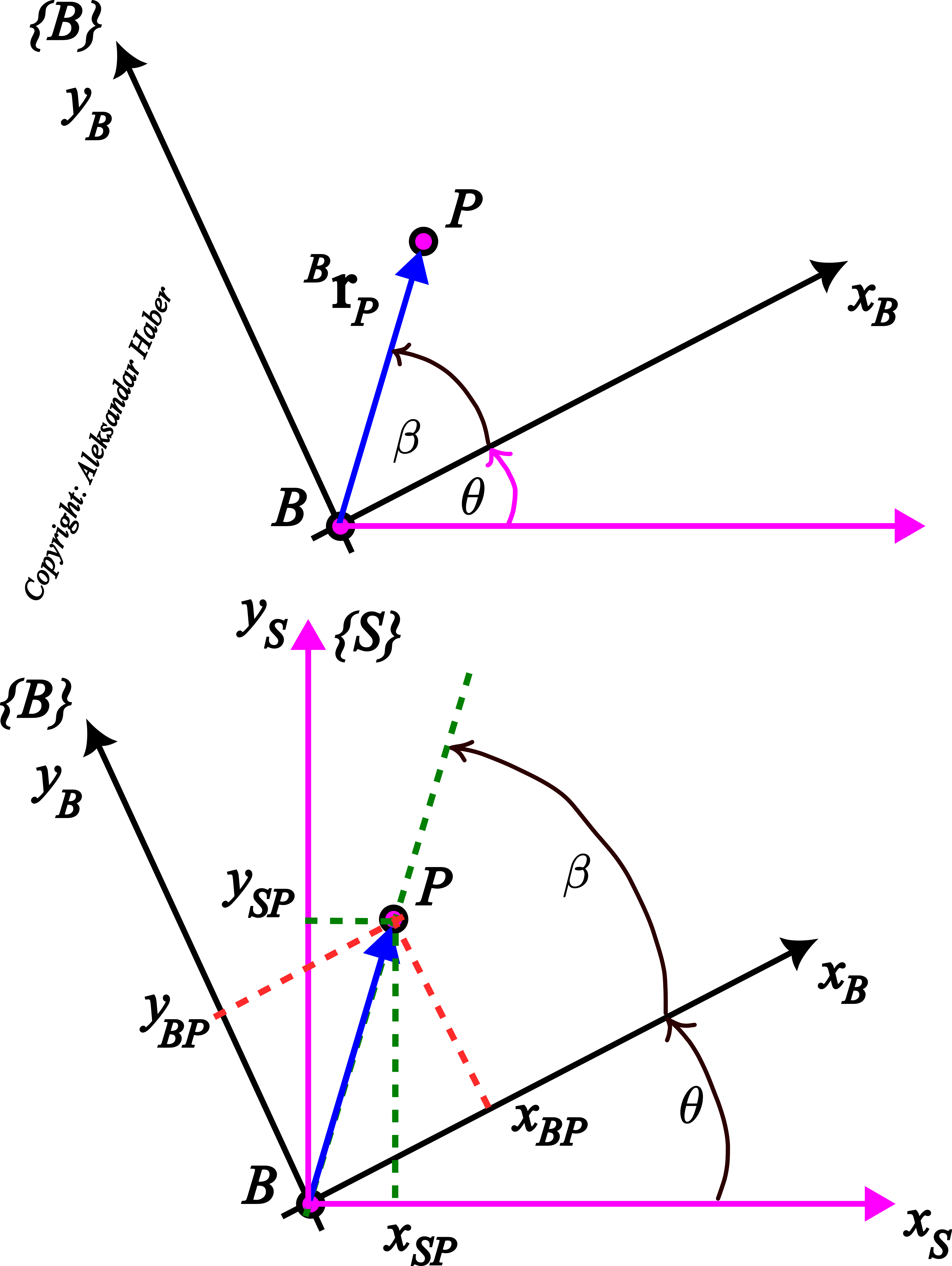Figure 2: Rotation of the frame $\{B \}$ for the angle of $\theta$ with respect to the frame $\{ S\}$ that is parallel to the fixed frame $\{F \}$ in Fig. 1.

The frame $\{S \}$ is fixed at the point $B$ and it cannot rotate. It is parallel to the frame $\{F \}$ . However, it can translate as the point $B$ translates. On the other hand, the frame $\{B \}$ is rotated for the angle $\theta$ with respect to the frame $\{S \}$ . Our first goal is to express the projections of the vector ${}^{B}\mathbf{r}_{P}$ in the frame $\{S \}$ . That is, we need to compute $x_{SP}$ and $y_{SP}$ (see the figure above). To do that, let us first denote the intensity of the vector ${}^{B}\mathbf{r}_{P}$ simply by $r$ . That is,

(6) $\begin{align*}r=|{}^{B}\mathbf{r}_{P} |\end{align*}$

We do that to simplify the notation. From the above figure, we have:

(7) $\begin{align*}x_{SP}& =r\cos(\theta+\beta) \\y_{SP}& =r\sin(\theta+\beta)\end{align*}$

where $\beta$ is the angle that the vector ${}^{B}\mathbf{r}_{P}$ creates with the axis $x_{B}$ . Next, let us recall the basic formula for the cosine and sine of two angles:

(8) $\begin{align*}\cos (\theta+\beta) =\cos (\theta) \cos (\beta) -\sin (\theta) \sin (\beta) \\\sin (\theta+\beta) =\sin (\theta) \cos(\beta)+\cos (\theta) \sin(\beta)\end{align*}$

By substituting these formulas in (7), we obtain

(9) $\begin{align*}x_{SP}& =r\cos(\theta+\beta)=r\cos (\theta) \cos (\beta) -r\sin (\theta) \sin (\beta) \\y_{SP}& =r\sin(\theta+\beta)=r\sin (\theta) \cos(\beta)+r\cos (\theta) \sin(\beta)\end{align*}$

Next, from Fig.2, it follows

(10) $\begin{align*}x_{BP}& =r\cos (\beta) \\y_{BP}& =r \sin(\beta)\end{align*}$

By substituting (10) in (9), we obtain

(11) $\begin{align*}x_{SP}& = \cos (\theta)x_{BP} -\sin (\theta) y_{BP} \\y_{SP}& =\sin (\theta) x_{BP}+ \cos (\theta) y_{BP} \end{align*}$

The last equation can be written in the matrix format

(12) $\begin{align*}\begin{bmatrix}x_{SP} \\y_{SP}\end{bmatrix} = \begin{bmatrix} \cos (\theta) & - \sin (\theta) \\ \sin (\theta) & \cos (\theta) \end{bmatrix}\begin{bmatrix} x_{BP} \\ y_{BP} \end{bmatrix}\end{align*}$

The last equation can be written compactly like this

(13) $\begin{align*}{}^{S}\mathbf{r}_{P} = {}^{S}_{B}R(\theta){}^{B}\mathbf{r}_{P}\end{align*}$

where

(14) $\begin{align*}{}^{S}\mathbf{r}_{P}=\begin{bmatrix}x_{SP} \\y_{SP}\end{bmatrix}, \; {}^{B}\mathbf{r}_{P}=\begin{bmatrix} x_{BP} \\ y_{BP} \end{bmatrix}, \; {}^{S}_{B}R(\theta)=\begin{bmatrix} \cos (\theta) & - \sin (\theta) \\ \sin (\theta) & \cos (\theta) \end{bmatrix}\end{align*}$

The matrix

(15) $\begin{align*}{}^{S}_{B}R(\theta)=\begin{bmatrix} \cos (\theta) & - \sin (\theta) \\ \sin (\theta) & \cos (\theta) \end{bmatrix}\end{align*}$

is called the rotation matrix. It transforms projections from the rotated frame $\{B \}$ to the frame $\{S \}$ . The subscript and superscript notation should be interpreted like that. The left superscript is the output frame and the left subscript is the input frame of the transformation.

The equation (13) is very important for the derivation of the homogeneous transforms. Namely, it tells us how to transform projections of a vector from the body frame to the frame that is parallel to the fixed frame. It tells us that we just need to multiply the projections in the body frame by the rotation matrix.

The second part of the solution: Derive the homogeneous transform matrix

Let us consider the Fig. 1 again. Below, Fig. 1 is repeated for clarity.

From this figure, we have

(16) $\begin{align*}{}^{F}\mathbf{r}_{P} = {}^{F}\mathbf{r}_{B}+ \Big[ {}^{B}\mathbf{r}_{P} \Big] \Bigg|_{\text{expressed in F}}\end{align*}$

where

(17) $\begin{align*}\Big[ {}^{B}\mathbf{r}_{P} \Big] \Bigg|_{\text{expressed in F}}\end{align*}$

is the vector ${}^{B}\mathbf{r}_{P}$ with the projections expressed in the frame $\{F \}$ . Since the axes of the frames $\{S \}$ and $\{ F\}$ are parallel, we have

(18) $\begin{align*}{}^{S}\mathbf{r}_{P} =\Big[ {}^{B}\mathbf{r}_{P} \Big] \Bigg|_{\text{expressed in F}}\end{align*}$

By substituting (18) in (16), we obtain

(19) $\begin{align*}{}^{F}\mathbf{r}_{P} = {}^{F}\mathbf{r}_{B}+{}^{S}\mathbf{r}_{P} \end{align*}$

By substituting (13) in (19), we obtain

(20) $\begin{align*}{}^{F}\mathbf{r}_{P} = {}^{F}\mathbf{r}_{B}+ {}^{S}_{B}R(\theta)\cdot {}^{B}\mathbf{r}_{P}\end{align*}$

On the other hand, since the axes of the frames $\{S \}$ and $\{F \}$ are parallel, we have

(21) $\begin{align*}{}^{S}_{B}R(\theta)={}^{F}_{B}R(\theta)\end{align*}$

By substituting (21) in (20), we have:

(22) $\begin{align*}{}^{F}\mathbf{r}_{P} = {}^{F}\mathbf{r}_{B}+ {}^{F}_{B}R(\theta)\cdot {}^{B}\mathbf{r}_{P}\end{align*}$

The last equation can be written compactly as a single matrix transform like this

(23) $\begin{align*}\begin{bmatrix} {}^{F}\mathbf{r}_{P} \\ 1 \end{bmatrix} =\begin{bmatrix}{}^{F}_{B}R(\theta) & {}^{F}\mathbf{r}_{B} \\ \mathbf{0}_{1\times 2} & 1 \end{bmatrix} \begin{bmatrix} {}^{B}\mathbf{r}_{P} \\ 1 \end{bmatrix} \end{align*}$

or in the expanded form

(24) $\begin{align*}\begin{bmatrix} x_{FP} \\y_{FP} \\ 1 \end{bmatrix} =\begin{bmatrix} \cos (\theta) & - \sin (\theta) & x_{FB} \\ \sin (\theta) & \cos (\theta) & y_{FB} \\ 0 & 0 & 1\end{bmatrix} \begin{bmatrix} x_{BP} \\ y_{BP} \\ 1 \end{bmatrix}\end{align*}$

We have solved the problem! We have derived the homogeneous transform matrix. From (23) and (24), we have that the homogeneous transform matrix has the following form:

(25) $\begin{align*}{}^{F}_{B}T=\begin{bmatrix}{}^{F}_{B}R(\theta) & {}^{F}\mathbf{r}_{B} \\ \mathbf{0}_{1\times 2} & 1 \end{bmatrix} = \begin{bmatrix} \cos (\theta) & - \sin (\theta) & x_{FB} \\ \sin (\theta) & \cos (\theta) & y_{FB} \\ 0 & 0 & 1\end{bmatrix} \end{align*}$

This matrix combines the rotation angle $\theta$ and the translation vector ${}^{F}\mathbf{r}_{B}$ in a single matrix transform! The equation (23) can be now written like this:

(26) $\begin{align*}\begin{bmatrix} {}^{F}\mathbf{r}_{P} \\ 1 \end{bmatrix} = {}^{F}_{B}T \begin{bmatrix} {}^{B}\mathbf{r}_{P} \\ 1 \end{bmatrix} \end{align*}$

and that is precisely the form (4) we were looking for in the problem formulation.

Copyright Notice and Notice not to Use By AI Algorithms for Training

Homogeneous Transform Problem Formulation

The first part of the solution: Derive the Rotation matrix

The second part of the solution: Derive the homogeneous transform matrix

admin

You might also like

How to Move and Jog an ABB Robot Using FlexPendant (Teach Pendant) – ABB Robotics Tutorial

Write Launch and URDF/XACRO Models Files and Load them in Gazebo

How to Draw Shear-Force and Bending-Moment Diagrams by Hand – Case of Concentrated Force (Concentrated Load)