In this control, robotics, and aerospace tutorial, we provide a clear and concise explanation of homogeneous transforms for robotics and aerospace engineering.
The main motivation for creating this tutorial comes from the fact that online and in some books there are incomplete or even incorrect explanations of homogeneous transforms. Consequently, a number of students and engineers do not properly understand the concept of homogeneous transforms. A proper understanding of homogenous transforms is very important for understanding the rigid body motion and for simulating the dynamics of rigid bodies. This tutorial is created to clarify everything. We have also created a YouTube lecture. The YouTube lecture is given below.

Homogeneous Transform Problem Formulation
For the presentation clarity, we consider a two-dimensional geometry. However, everything explained in this tutorial can easily be generalized to three-dimensional geometry. Consider the geometry shown in the figure below.

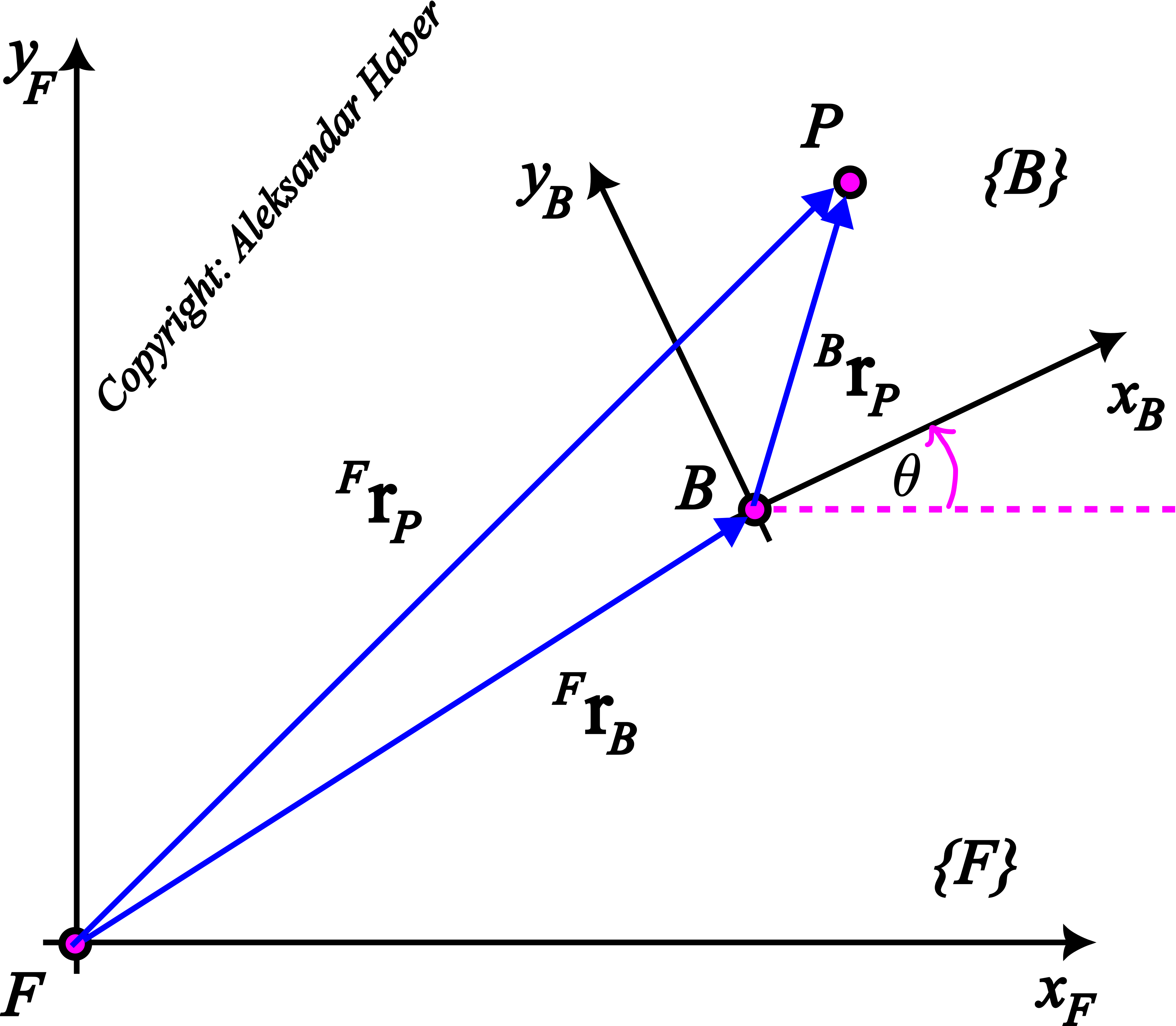
Essentially, this figure shows two coordinate frames (coordinate systems): 


The notation used in the figure is explained below:
- The points


- The vector denoted by


- The vector denoted by

- The vector denoted by

- The angle


Let us introduce the notation for the projections of the vector
(1) 

where 


Let us introduce the notation for the projections of the vector
(2) 

where 


Finally, let us introduce the notation for the projections of the vector
(3) 
where 

The Homogeneous Transform Problem can be formulated as follows. Given
- Coordinates of the point

- The angle of rotation
- The vector
determine the matrix 

(4) 

or
(5) 

In other words, our goal is to determine the transformation matrix 

The matrix
The first part of the solution: Derive the Rotation matrix
To solve this problem, we first need to derive the rotation matrix transforming the coordinates from 


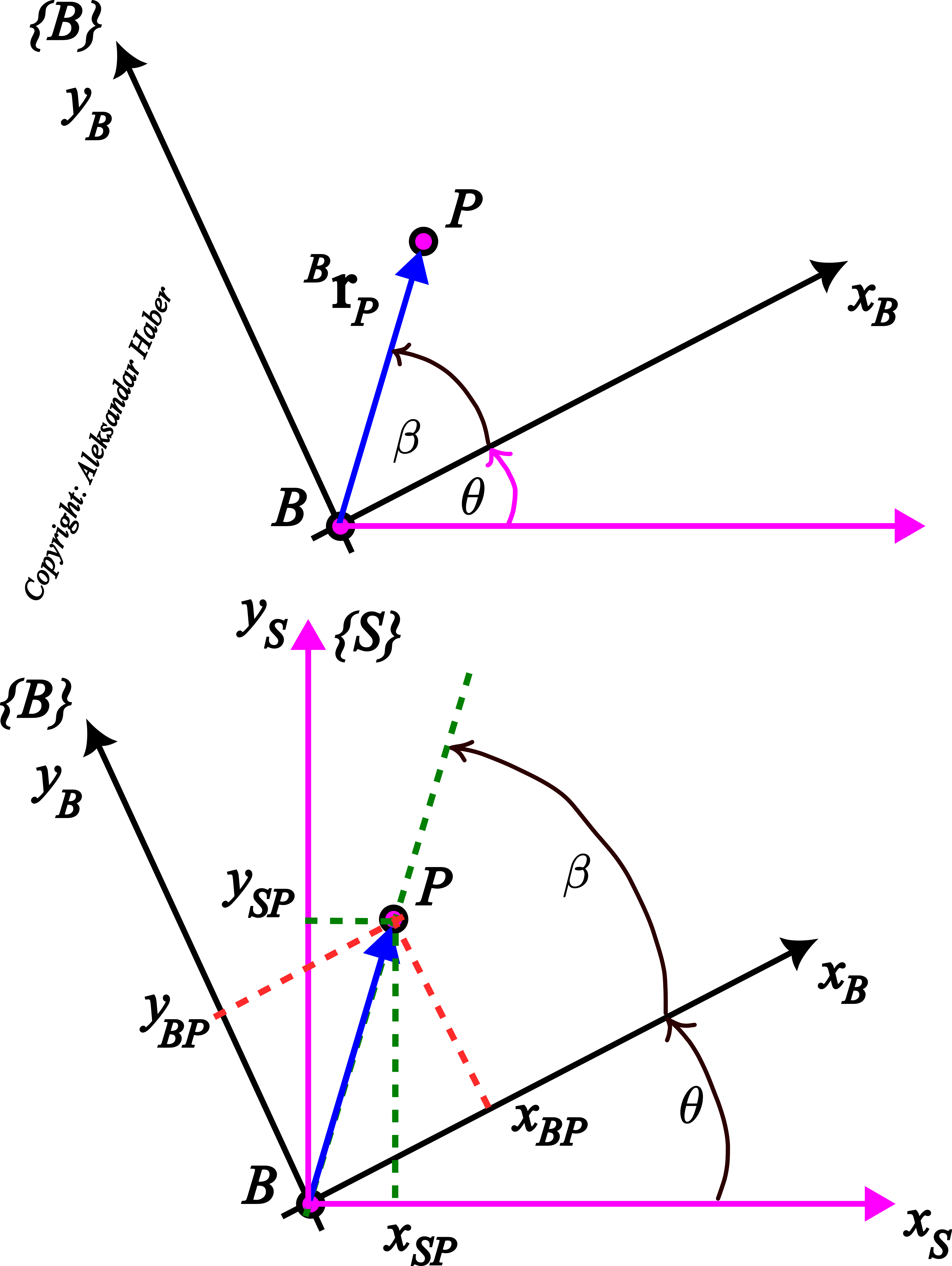
The frame 


(6) 

We do that to simplify the notation. From the above figure, we have:
(7) 

where 

(8) 

By substituting these formulas in (7), we obtain
(9) 

Next, from Fig.2, it follows
(10) 

By substituting (10) in (9), we obtain
(11) 

The last equation can be written in the matrix format
(12) 

The last equation can be written compactly like this
(13) 

where
(14) 

The matrix
(15) 

is called the rotation matrix. It transforms projections from the rotated frame
The equation (13) is very important for the derivation of the homogeneous transforms. Namely, it tells us how to transform projections of a vector from the body frame to the frame that is parallel to the fixed frame. It tells us that we just need to multiply the projections in the body frame by the rotation matrix.
The second part of the solution: Derive the homogeneous transform matrix
Let us consider the Fig. 1 again. Below, Fig. 1 is repeated for clarity.
From this figure, we have
(16) ![\begin{align*}{}^{F}\mathbf{r}_{P} = {}^{F}\mathbf{r}_{B}+ \Big[ {}^{B}\mathbf{r}_{P} \Big] \Bigg|_{\text{expressed in F}}\end{align*}](https://aleksandarhaber.com/wp-content/ql-cache/quicklatex.com-8e238b57a5aae4b569a6a190590473a3_l3.png "Rendered by QuickLaTeX.com")

where
(17) ![\begin{align*}\Big[ {}^{B}\mathbf{r}_{P} \Big] \Bigg|_{\text{expressed in F}}\end{align*}](https://aleksandarhaber.com/wp-content/ql-cache/quicklatex.com-fb4cdefb2ea27cecbe34d87a69a2c6ee_l3.png "Rendered by QuickLaTeX.com")

is the vector
(18) ![\begin{align*}{}^{S}\mathbf{r}_{P} =\Big[ {}^{B}\mathbf{r}_{P} \Big] \Bigg|_{\text{expressed in F}}\end{align*}](https://aleksandarhaber.com/wp-content/ql-cache/quicklatex.com-f38432af7cfbf47c1072c151764d6e7a_l3.png "Rendered by QuickLaTeX.com")

By substituting (18) in (16), we obtain
(19) 

By substituting (13) in (19), we obtain
(20) 

On the other hand, since the axes of the frames
(21) 

By substituting (21) in (20), we have:
(22) 
The last equation can be written compactly as a single matrix transform like this
(23) 

or in the expanded form
(24) 

We have solved the problem! We have derived the homogeneous transform matrix. From (23) and (24), we have that the homogeneous transform matrix has the following form:
(25) 

This matrix combines the rotation angle
(26) 

and that is precisely the form (4) we were looking for in the problem formulation.