Python Control Systems Lecture 2: Transfer Function Definition and Simulation of Step, Impulse, and User-Defined Input Responses

In this Python control systems tutorial, we explain how to define transfer functions and how to simulate step, impulse, and user-defined input responses. For that purpose, we use the Python control systems library. The YouTube tutorial is given below.

Copyright notice

Copyright notice: this lesson, developed code files, and documents should not be copied, redistributed, or posted on public or private websites, public or private code repositories, or social media platforms. This lesson and all the provided study materials are strictly for personal use. Without the permission of the author, this lesson and the provided material should not be used for commercial purposes and for training of engineers working in companies. This lesson and the provided material should not be used as lecture materials on online learning platforms and in university courses. This lesson and the provided material should not be used to train an AI algorithm or a large language model.

Prerequisites

To implement the material presented in this lecture you need to install the Python Control Systems, NumPy, and Matplotlib libraries. Consequently, you need to run these pip install commands:

pip install numpy 
pip install matplotlib
pip install 

Transfer Function Definition and Responses

First, we need to import the necessary libraries

import matplotlib.pyplot as plt
import control as ct
import numpy as np

Here, we import the control systems library “control” as “ct”. Next, we define the plotting function that we will use in this tutorial to plot the responses.

# this function is used for plotting of responses 
# it generates a plot and saves the plot in a file 

# xAxisVector - time vector
# yAxisVector - response vector
# titleString - title of the plot
# stringXaxis - x axis label 
# stringYaxis - y axis label
# stringFileName - file name for saving the plot, usually png or pdf files

def plottingFunction(xAxisVector,yAxisVector,titleString,stringXaxis,stringYaxis,stringFileName):
    plt.figure(figsize=(8,6))
    plt.plot(xAxisVector,yAxisVector, color='blue',linewidth=4)
    plt.title(titleString, fontsize=14)
    plt.xlabel(stringXaxis, fontsize=14)
    plt.ylabel(stringYaxis,fontsize=14)
    plt.tick_params(axis='both',which='major',labelsize=14)
    plt.grid(visible=True)
    plt.savefig(stringFileName,dpi=600)
    plt.show()

Next, we explain how to define transfer functions. To define a transfer function, let us consider this example

(1)  

We define this transfer function like this

# define a transfer function
num=[2,4]
den=[1,2,4]

# here we define the transfer function
W=ct.tf(num,den)
print(W)

That is, first we defined two lists storing the coefficients of the polynomials in the numerator and denominator of the transfer function. The first list called “num” stores the coefficients of the polynomial in the numerator. The second list called “den” stores the coefficients of the polynomial in the denominator. To define the transfer function, we use the “tf” function. We pass the two lists as input parameters. This function returns a transfer function object that can be used for simulations.

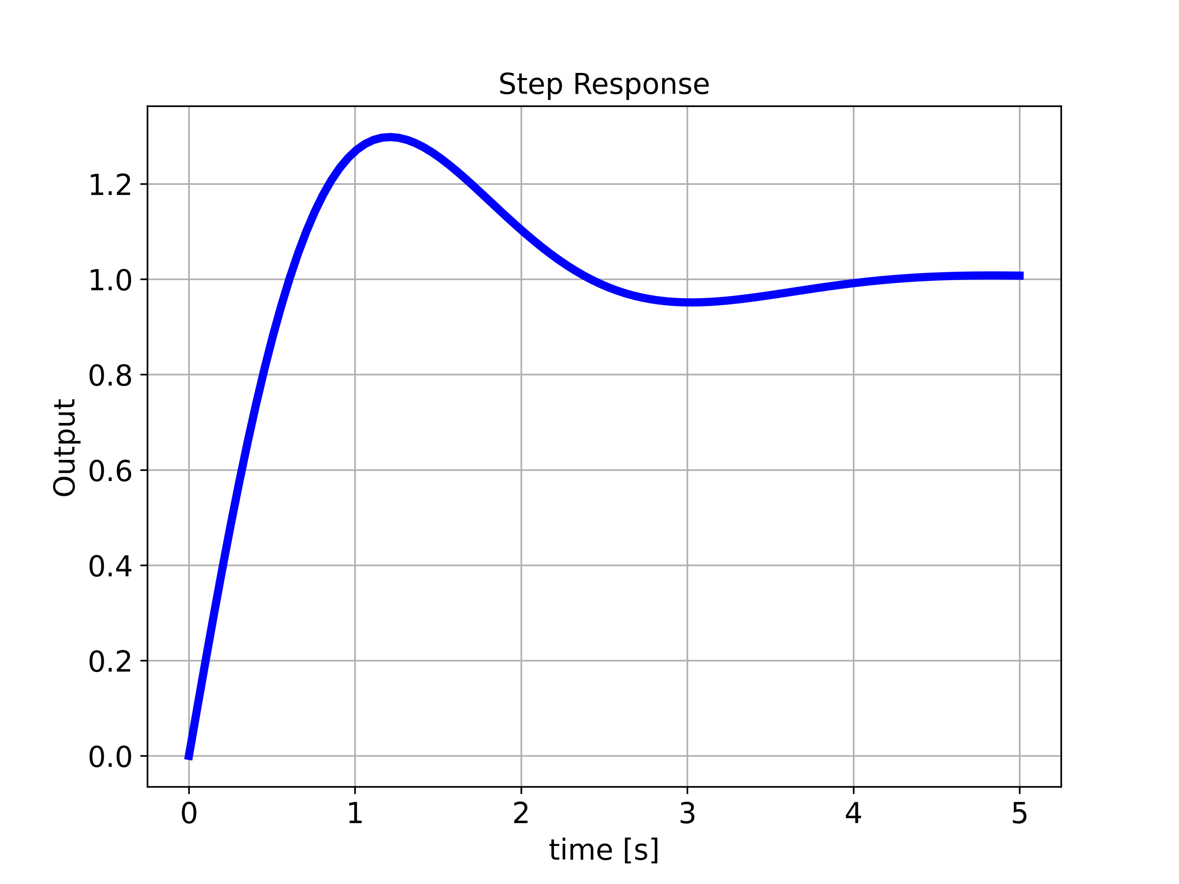
The following code block simulates the step response of the system

###############################################################################
# simulate the step response
###############################################################################
timeVector=np.linspace(0,5,100)
timeReturned, systemOutput = ct.step_response(W,timeVector)

# plot the step response
plottingFunction(timeReturned,systemOutput,
                 titleString='Step Response',
                 stringXaxis='time [s]' , 
                 stringYaxis='Output',
                 stringFileName='stepResponseNew.png',)
###############################################################################

To simulate the step response, we use the function “step_response()”. The first input parameter is the transfer function object, and the second input parameter is the time vector for simulation. This function simulates the step response and returns the simulation time and the simulated response. Next, we plot the step response. The step response is shown in the figure below.

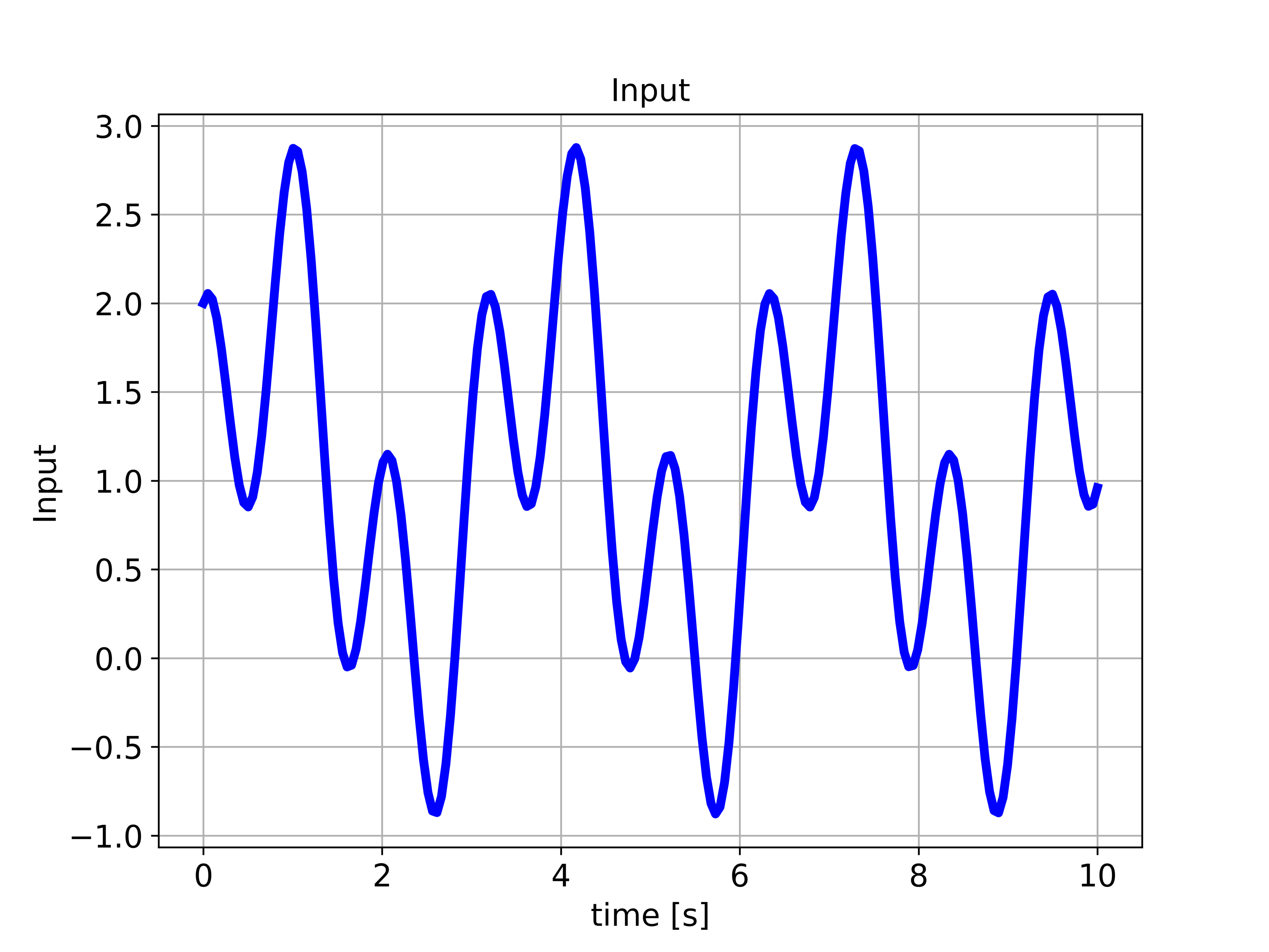
The code block shown below simulates the response of the system to a user-defined input:

###############################################################################
# Simulate the system response to a specific input
###############################################################################
# generate the input vector
timeVector2=np.linspace(0,10,200)
inputVector2=np.sin(2*timeVector2)+np.cos(6*timeVector2)+np.ones(timeVector2.shape)

# initial state
x0=np.array([[0],[0]])

# plot the input vector
plottingFunction(timeVector2,inputVector2,
                 titleString='Input',
                 stringXaxis='time [s]' , 
                 stringYaxis='Input', 
                 stringFileName='appliedInput.png')

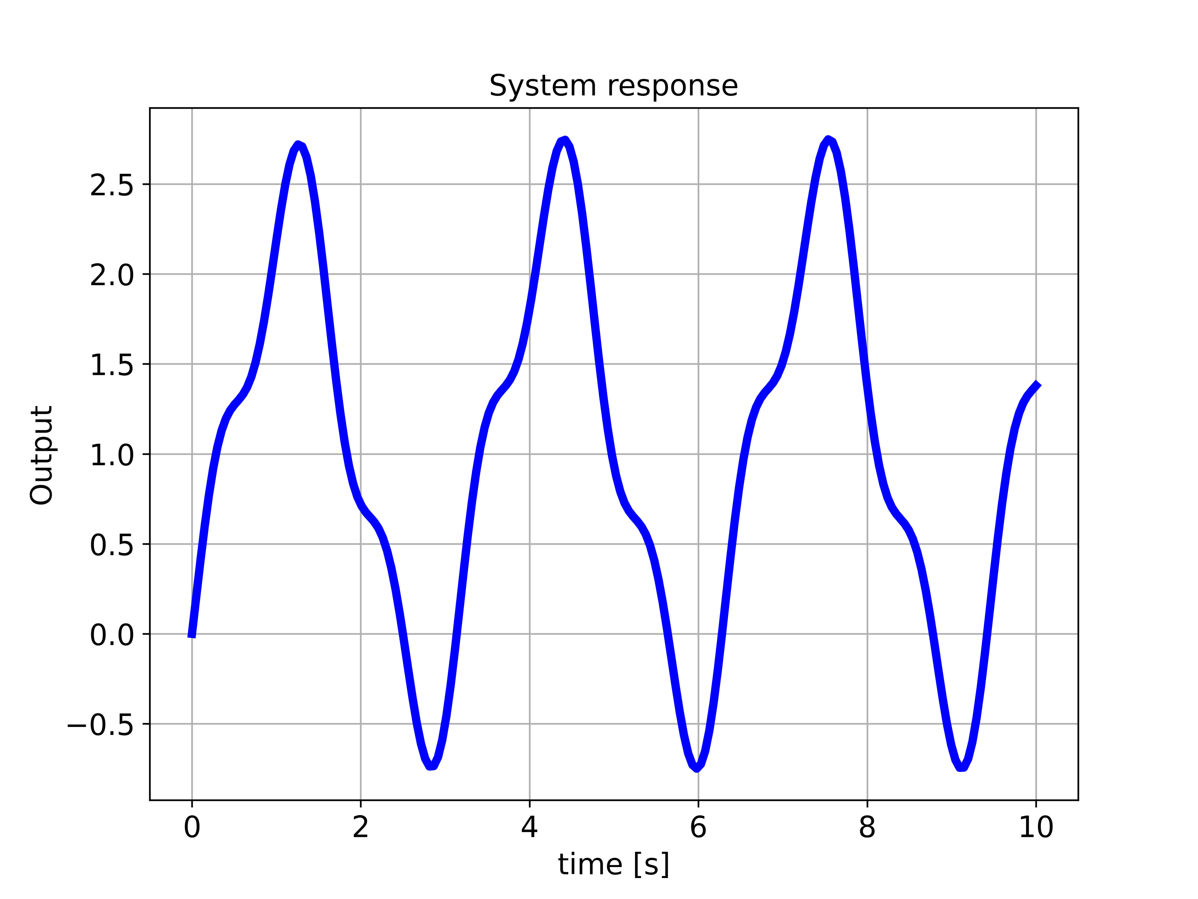
# compute the response of the system to the specific input
timeReturned2, systemOutput2 = ct.forced_response(W,timeVector2,inputVector2)
plottingFunction(timeReturned2,systemOutput2,
                 titleString='System response',
                 stringXaxis='time [s]' , 
                 stringYaxis='Output', 
                 stringFileName='outputSinusoidal.png')
###############################################################################

First, we define the control input. Secondly, we compute the response to this user-defined input, by using the function “forced_response”. The first input parameter is the transfer function object. The second input parameter is the time vector and the third input parameter is the control input vector. We plot the control input and the simulated response. The graphs are given below.

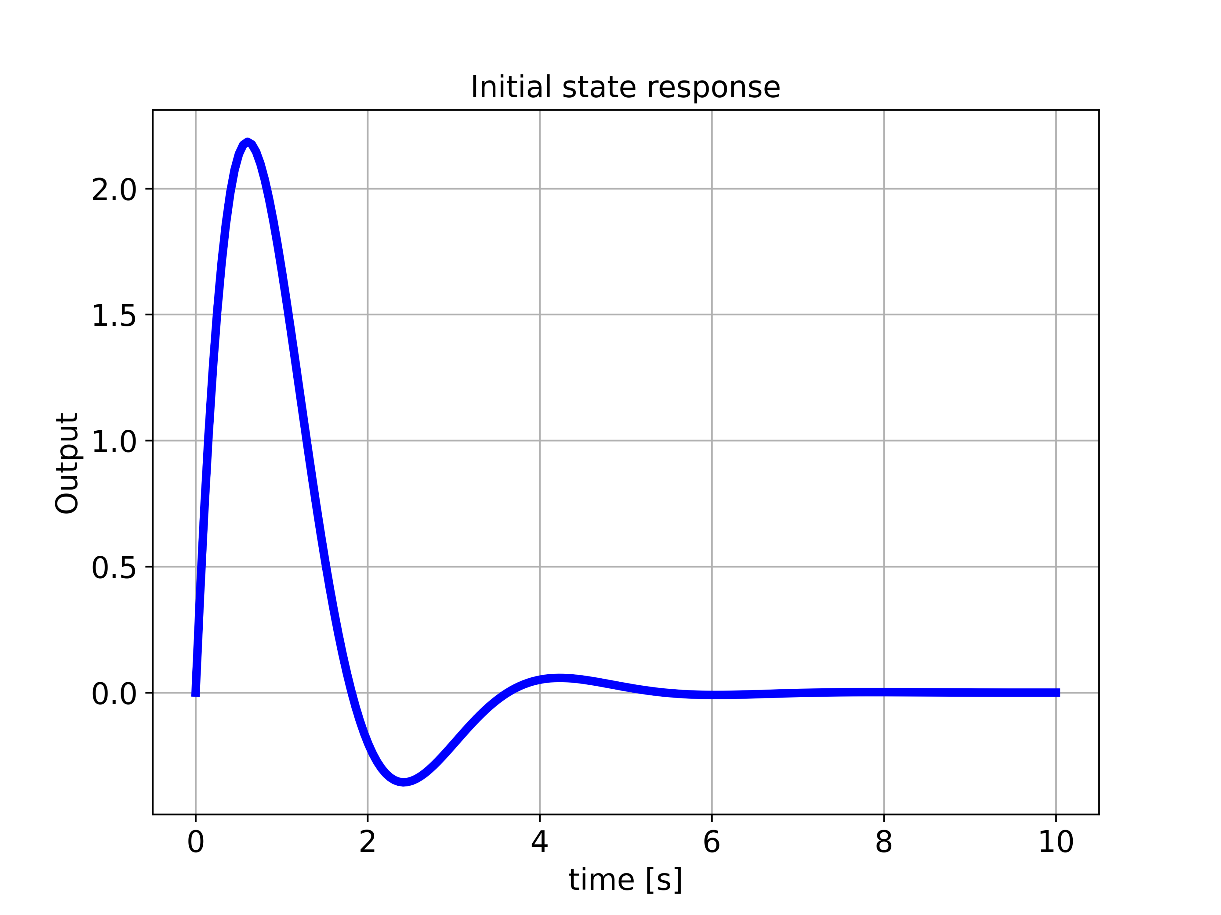
We compute the initial state response of the system by using the code block shown below.

###############################################################################
# Initial state response
###############################################################################
timeVector3=np.linspace(0,10,200)
initialState=np.array([2,-1])

timeReturned3, systemOutput3 = ct.initial_response(W,timeVector3,initialState)
plottingFunction(timeReturned3,systemOutput3,
                 titleString='Initial state response',
                 stringXaxis='time [s]' , 
                 stringYaxis='Output', 
                 stringFileName='outputInitial.png')

The response is given in the figure below.

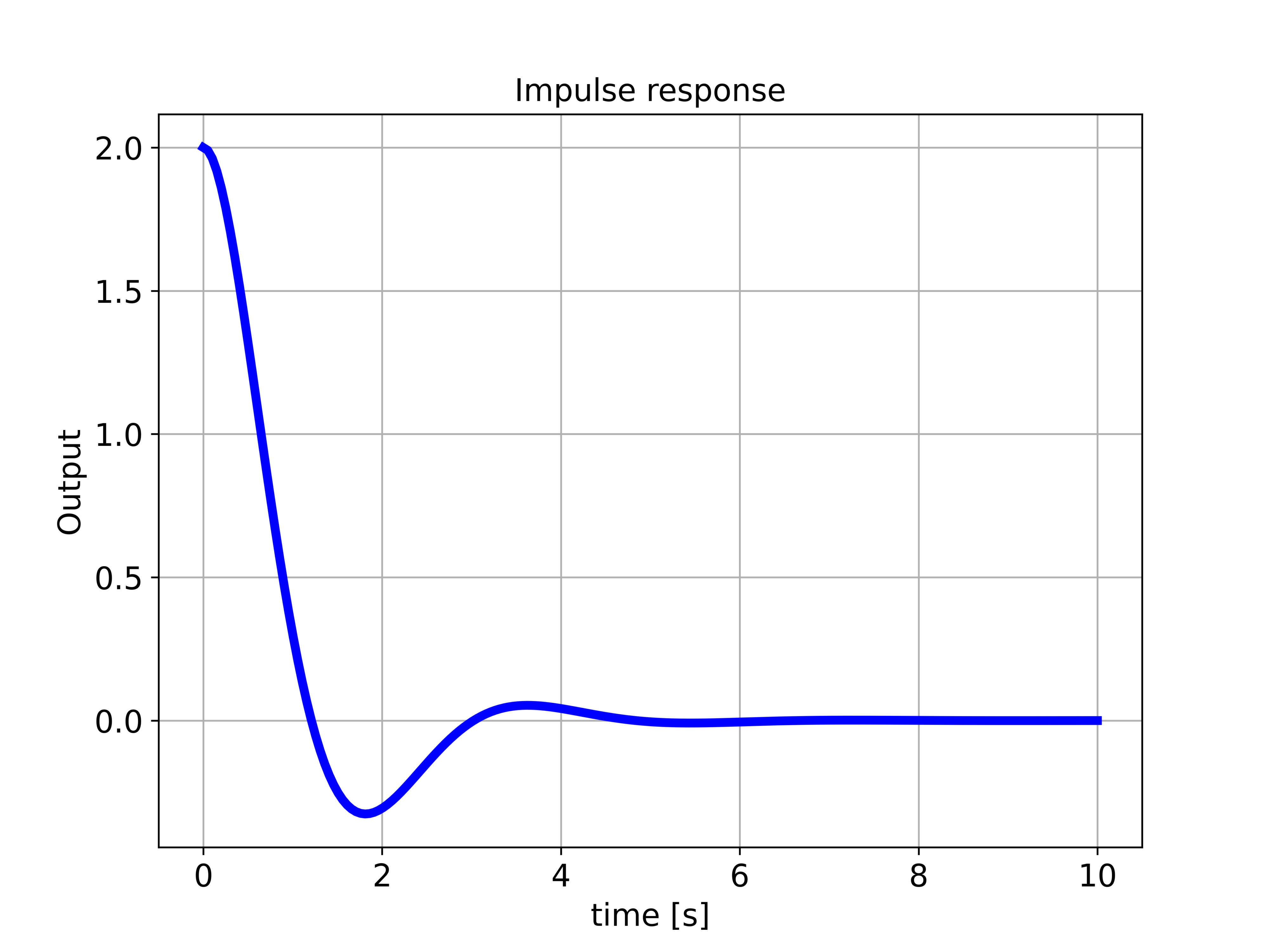
The impulse response is simulated by using the code given below.

###############################################################################
# Impulse response
###############################################################################

timeVector4=np.linspace(0,10,200)

timeReturned4, systemOutput4 = ct.impulse_response(W,timeVector4)
plottingFunction(timeReturned4,systemOutput4,
                 titleString='Impulse response',
                 stringXaxis='time [s]' , 
                 stringYaxis='Output', 
                 stringFileName='outputImpulse.png')

The impulse response is shown in the figure below.