How to simulate responses of state-space models to arbitrary control inputs in MATLAB – Control Engineering Tutorial – Fusion of Engineering, Control, Coding, Machine Learning, and Science

In this tutorial, we explain how to simulate responses of state-space models to arbitrary control inputs in MATLAB. We first explain how to define a state-space model in MATLAB. After that, we define an arbitrary control input, and we simulate the state-space model for the defined control input in MATLAB. The YouTube tutorial accompanying this post is given below.

As a test case, in this tutorial, we consider a second-order mass-spring-damper system whose dynamics is derived by applying Newton’s second law. The dynamics is described by the following ordinary differential equation

(1) $\begin{align*}m\ddot{x}+k_{d}\dot{x}+k_{s}x=F\end{align*}$

where $m$ is the mass, $k_{d}$ is the damping constant, $k_{s}$ is the spring constant, $x$ is the displacement of the mass, $\dot{x}$ is the first time derivative of $x$ , and $\ddot{x}$ is the second time derivative of $x$ . The force $F$ acts as a control input. By assigning the state-space variables

(2) $\begin{align*}\mathbf{x}=\begin{bmatrix} x_{1} \\ x_{2} \end{bmatrix}\end{align*}$

from (1), we obtain a state space model

(3) $\begin{align*}\dot{\mathbf{x}}& =A\mathbf{x}+B\mathbf{u}\\\mathbf{y}&=C\mathbf{x}+D\mathbf{u}\end{align*}$

where

(4) $\begin{align*}& A=\begin{bmatrix}0 & 1 \\ -\frac{k_{s}}{m} & -\frac{k_{d}}{m} \end{bmatrix} \\& B=\begin{bmatrix} 0 \\ \frac{1}{m} \end{bmatrix} \\& C=\begin{bmatrix} 1 & 0 \end{bmatrix} \\& D=0\end{align*}$

First, we need to define the model parameters and the state-space model. We use the MATLAB code given below to perform these tasks:

clear, clc 

m=0.1
ks=5
kd=0.01

A=[0 1; 
    -ks/m -kd/m];
B=[0; 1/m];
C=[1 0];
D=0

ssModel=ss(A,B,C,D);

To define the state-space model, we use MATLAB’s function ss(). The input arguments of this function are the system matrices. Next, we need to define the input for the simulation:


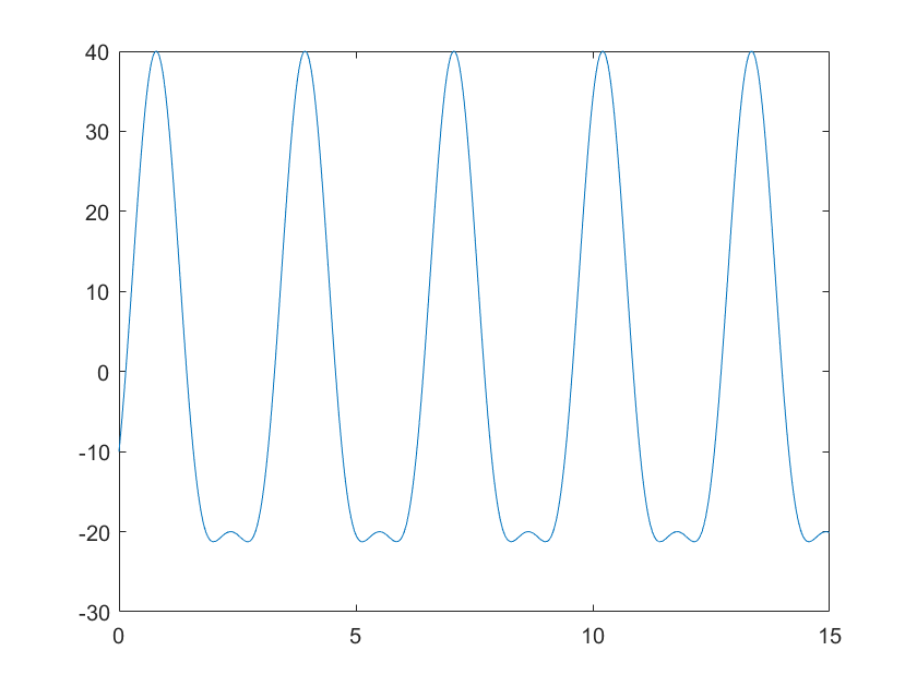
time=0:0.01:15

controlU=30*sin(2*time)-10*cos(4*time)

figure(1)
plot(time, controlU)

The input is shown in the figure below.

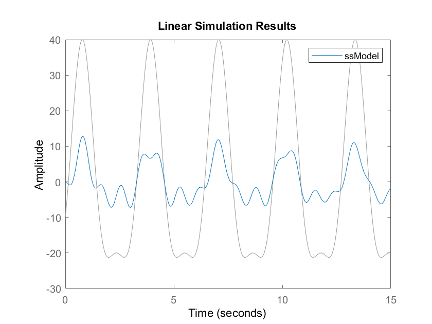
Fig. 1: Input for simulating the state-space model.

To simulate the state-space model for this input, we use MATLAB’s function lsim():


figure(2)
lsim(ssModel,controlU,time)

The first input argument of lsim() is the defined state-space model. The second input argument is the vector defining the control input as a function of a discrete time, and the final control input is the time vector that is used to define the control input. The generated response is shown in the figure below.

Fig. 2: Simulated output (blue line) and control input (grey line).

Often, it is necessary to extract the numerical values of the simulated response, we can do that by explicitly specifying the outputs of the lsim() function. The lsim() function will return the simulated output and the time vector used to simulate the output. The code given below will return the time series of the simulated output and it will plot the simulated output in a new figure.


[ys,ti]=lsim(ssModel,controlU,time)

figure(3)
plot(ti,ys)

Finally, in the lsim() function, as the last argument, we can specify the initial condition for the simulation:

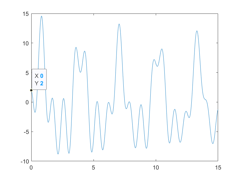
X0=[2; -2]

[ys2,ti2]=lsim(ssModel,controlU,time,X0)
figure(4)
plot(ti2,ys2)

The simulated output for the specified initial condition is shown in the figure below.

admin

You might also like

Lyapunov Equation: How to Compute the Solution and Origins in Stability Analysis of Dynamical Systems

Implementation of the Solution of the Linear Quadratic Regulator (LQR) Control Algorithm in C++ by Using the Eigen Matrix Library

Dynamical Model of a Tank (Reservoir) Filled with Liquid and Simulation in Python