Frequency Response and Bode Plot of an RC circuit – Fusion of Engineering, Control, Coding, Machine Learning, and Science

In this electrical engineering tutorial we explain how to derive a frequency response and a Bode plot of an RC (resistor-capacitor) circuit. As it will be explained in this tutorial, the RC circuit constitutes a low-pass filter. The YouTube tutorial is given below.

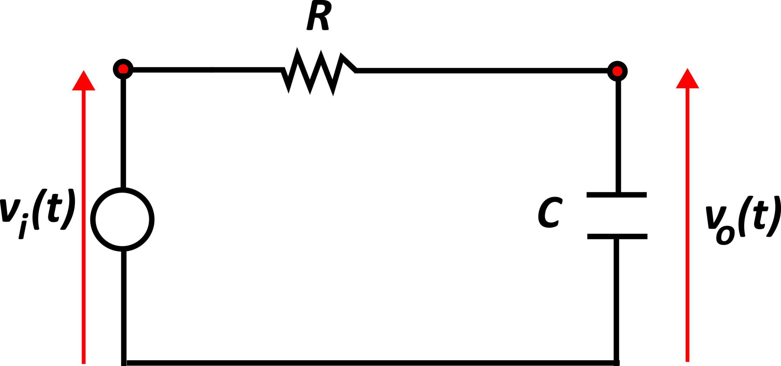
Consider the RC circuit shown below. The circuit consists of the resistor with the resistance of $R$ , voltage source, and the capacitor with the capacitance of $C$ . The input and output voltages are denoted by $v_{i}(t)$ and $v_{o}(t)$ .

We first need to derive a transfer function of this circuit from the input to the output voltages. To derive the transfer function, we use the impedance approach. We transform the circuit shown above in the complex $s$ domain. The resistor and capacitor are replaced by the corresponding impedances, and the voltages are replaced by the Laplace transforms of voltages. The transformed circuit is shown below.

In the figure above, the impedance $Z_{1}(s)$ is the impedance of the resistor. This impedance is given by

(1) $\begin{align*}Z_{1}(s)=R\end{align*}$

The impedance $Z_{2}(s)$ is the impedance of the capacitor. This impedance is given by

(2) $\begin{align*}Z_{2}(s)=\frac{1}{Cs}\end{align*}$

The Laplace transform of $v_{i}(t)$ is denoted by $V_{i}(s)$ . The Laplace transform of $v_{o}(t)$ is denoted by $V_{o}(s)$ .

By using the Ohm’s law in the complex Laplace domain, we obtain

(3) $\begin{align*}\frac{V_{i}-V_{o}}{Z_{1}}=\frac{V_{o}}{Z_{2}}\end{align*}$

where for notation simplicity, we drop out the dependence of variables on $s$ . From the last equation, we have

(4) $\begin{align*}(V_{i}-V_{o})Z_{2}=V_{o}Z_{1} \\V_{i}Z_{2}=V_{o}(Z_{1}+Z_{2})\end{align*}$

From the last equation, we obtain

(5) $\begin{align*}\frac{V_{o}}{V_{i}}=\frac{Z_{2}}{Z_{1}+Z_{2}}\end{align*}$

By substituting the impedances in the last equation, we obtain

(6) $\begin{align*}\frac{V_{o}}{V_{i}}=\frac{\frac{1}{Cs}}{R+\frac{1}{Cs}}=\frac{1}{1+RCs}\end{align*}$

Frequency Response Derivation

Let us denote the transfer function by $W(s)$

(7) $\begin{align*}W(s)=\frac{1}{1+RCs}\end{align*}$

The frequency response consists of the magnitude and phase response. By substituting $s=\omega j$ in (7), where $\omega$ is the angular frequency and $j$ is the imaginary unit, we have

(8) $\begin{align*}W(\omega j)=\frac{1}{1+RC\omega j}\end{align*}$

The last equation defines a complex number. By writing this number in the polar form, we obtain

(9) $\begin{align*}W(\omega j)=\frac{1}{1+RC\omega j}=\frac{1}{\sqrt{1+R^{2}C^{2}\omega^2}}e^{-j \arctan (RC\omega)}\end{align*}$

From the last equation, we obtain the magnitude $M(\omega)$ and phase responses $\phi (\omega)$

(10) $\begin{align*}M(\omega) & =\frac{1}{\sqrt{1+R^{2}C^{2}\omega^2}} \\\phi (\omega) & = -\arctan (RC\omega)\end{align*}$

The break frequency (also known as the cutoff or corner frequency) is given for the frequency where

(11) $\begin{align*}M(\omega_{c})=\frac{1}{\sqrt{2}}\end{align*}$

We can observe that the break frequency is

(12) $\begin{align*}\omega_{c} & = \frac{1}{RC} \\f_{c}&= \frac{1}{2\pi \cdot RC}\end{align*}$

The Bode plot is a plot of the log-magnitude response given by

(13) $\begin{align*}L = 20 \text{log} (M(\omega)) = 20 \text{log} ( \frac{1}{\sqrt{1+R^{2}C^{2}\omega^2}} ) = - 20 \text{log} ( \sqrt{1+R^{2}C^{2}\omega^2} )\end{align*}$

and the phase response defined by

(14) $\begin{align*}\phi (\omega) & = -\arctan (RC\omega)\end{align*}$

Frequency Response Derivation

admin

You might also like

Compute Magnitude and Phase Responses (Frequency Response) of Digital Filters and Discrete-Time Systems in Python

Control Systems Lecture: Simulation of linear ordinary differential equations using Python and state-space modeling

Nonlinear Model Predictive Control – MPC – Tutorial 1: Basic Formulation and Solution in MATLAB