Python Control Systems Lecture 3: Definition of State-space Models and Simulation in Python

In this tutorial, we use Python and Python Control Systems Library. We explain how to

• Define a state-space model
• Simulate and plot the step response
• Simulate and plot the response to arbitrary inputs
• Transform state-space models to transfer functions and back
• Discretize state-space models
• Investigate the dynamic properties of state-space models

The YouTube tutorial is given below.

Copyright notice: this video lesson, developed code files, and documents should not be copied, redistributed, or posted on public or private websites, public or private code repositories, or social media platforms. This lesson and all the provided study materials are strictly for personal use. Without the permission of the author, this lesson and the provided material should not be used for commercial purposes and for training of engineers working in companies. This lesson and the provided material should not be used as lecture materials on online learning platforms and in university courses. This lesson and the provided material should not be used to train an AI algorithm or a large language model.

Import Libraries and Define Python Function

You need to install NumPy, Control System, and Matplotlib Python libraries. You can do that in the Python terminal by typing

pip install numpy 
pip install control
pip install matplotlib

Let us explain the Python code. First, we need to import the necessary libraries, and to defined a plotting function. The following Python scripts imports Numpy, Control, and Matplotlib libraries and defines a plotting function.

import matplotlib.pyplot as plt
import control as ct
import numpy as np

# this function is used for plotting of responses 
# it generates a plot and saves the plot in a file 

# xAxisVector - time vector
# yAxisVector - response vector
# titleString - title of the plot
# stringXaxis - x axis label 
# stringYaxis - y axis label
# stringFileName - file name for saving the plot, usually png or pdf files

def plottingFunction(xAxisVector,yAxisVector,titleString,
                     stringXaxis,stringYaxis,stringFileName):
    plt.figure(figsize=(8,6))
    plt.plot(xAxisVector,yAxisVector, color='blue',linewidth=4)
    plt.title(titleString, fontsize=14)
    plt.xlabel(stringXaxis, fontsize=14)
    plt.ylabel(stringYaxis,fontsize=14)
    plt.tick_params(axis='both',which='major',labelsize=14)
    plt.grid(visible=True)
    plt.savefig(stringFileName,dpi=600)
    plt.show()

The plotting function generates the plot and saves the plot in a specified png or jpeg file. This will be explained later on in this tutorial.

Define State-Space Models in Python

In this tutorial, we use the following example of a state-space model

(1)  

To define a state-space model in Python, we need to specify system matrices as numpy arrays, and use the function “ct.ss”:

A=np.array([[0,1],[-4,-2]])
B=np.array([[0],[1]])
C=np.array([[1,0]])
D=np.array([[0]])

sysState=ct.ss(A,B,C,D)

print(sysState)

Convert State-space Models to Transfer Functions and Back in Python

To convert state-space models to transfer function models, we use the function “ct.ss2tf()”. On the other hand, to convert transfer functions to state-space models, we use the function “ct.tf2ss()”. The code is given below.

# convert to tf 

transferFunction1=ct.ss2tf(sysState)

print(transferFunction1)

sysState2=ct.tf2ss(transferFunction1)

Simulate the Step Response of a State-Space Model in Python

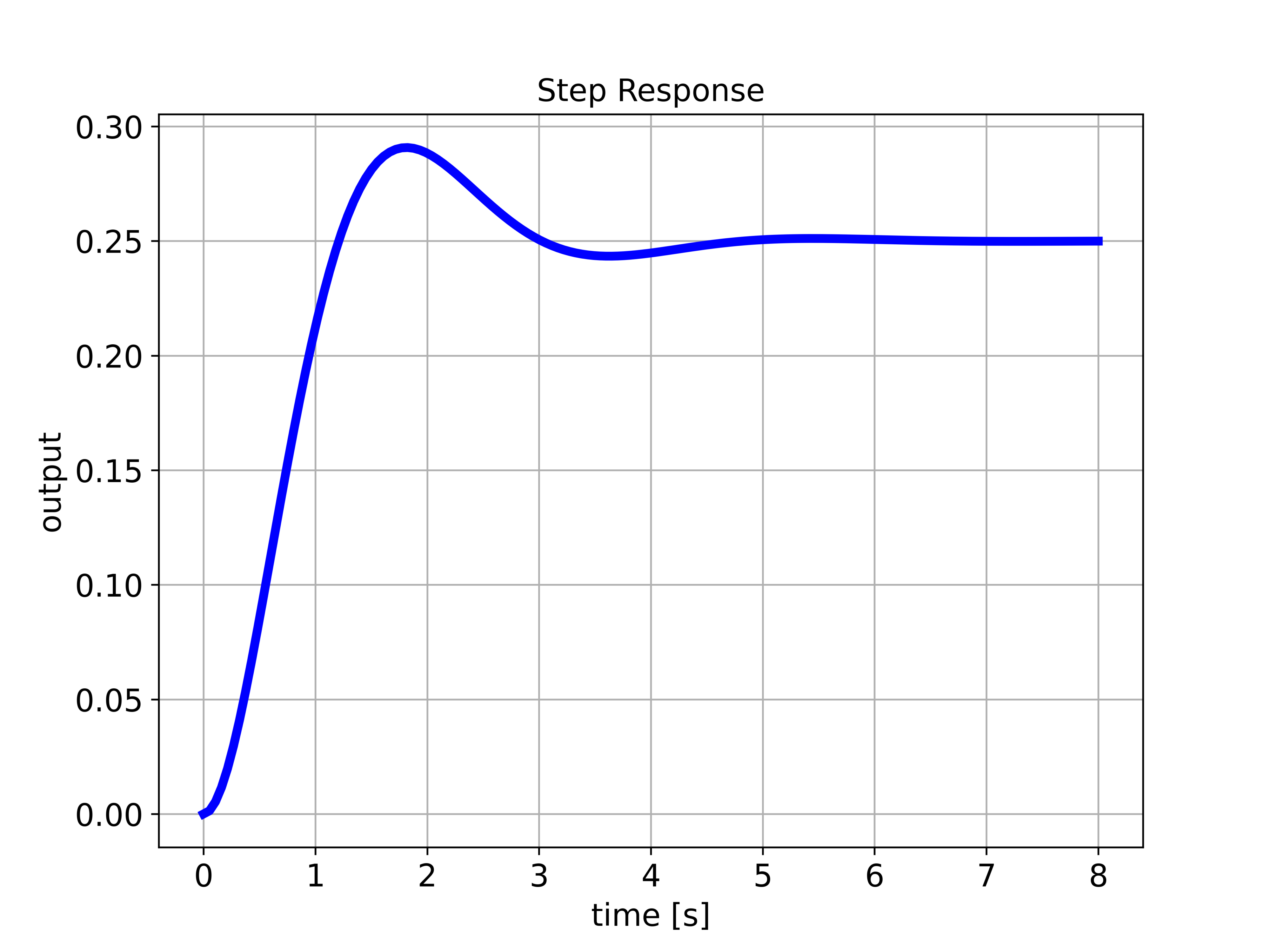
To simulate the step response of a state-space model, we first need to define a time vector used for simulation. After that, we need to use the function “ct.step_response()”. The first input parameter is the state-space model object, and the second input parameter is the time vector. The function “ct.step_response()” returns the time vector used for simulation and the computed step response. The code given below computes and plots the step response by using the previously defined function:

timeVector=np.linspace(0,8,150)

timeReturned,systemOutput=ct.step_response(sysState,timeVector)

plottingFunction(timeReturned,systemOutput,'Step Response',
                     'time [s]','output','stepResponse.png')

The step response is given in the figure below.

Simulate the Response of a State-Space Model to User Defined Input in Python

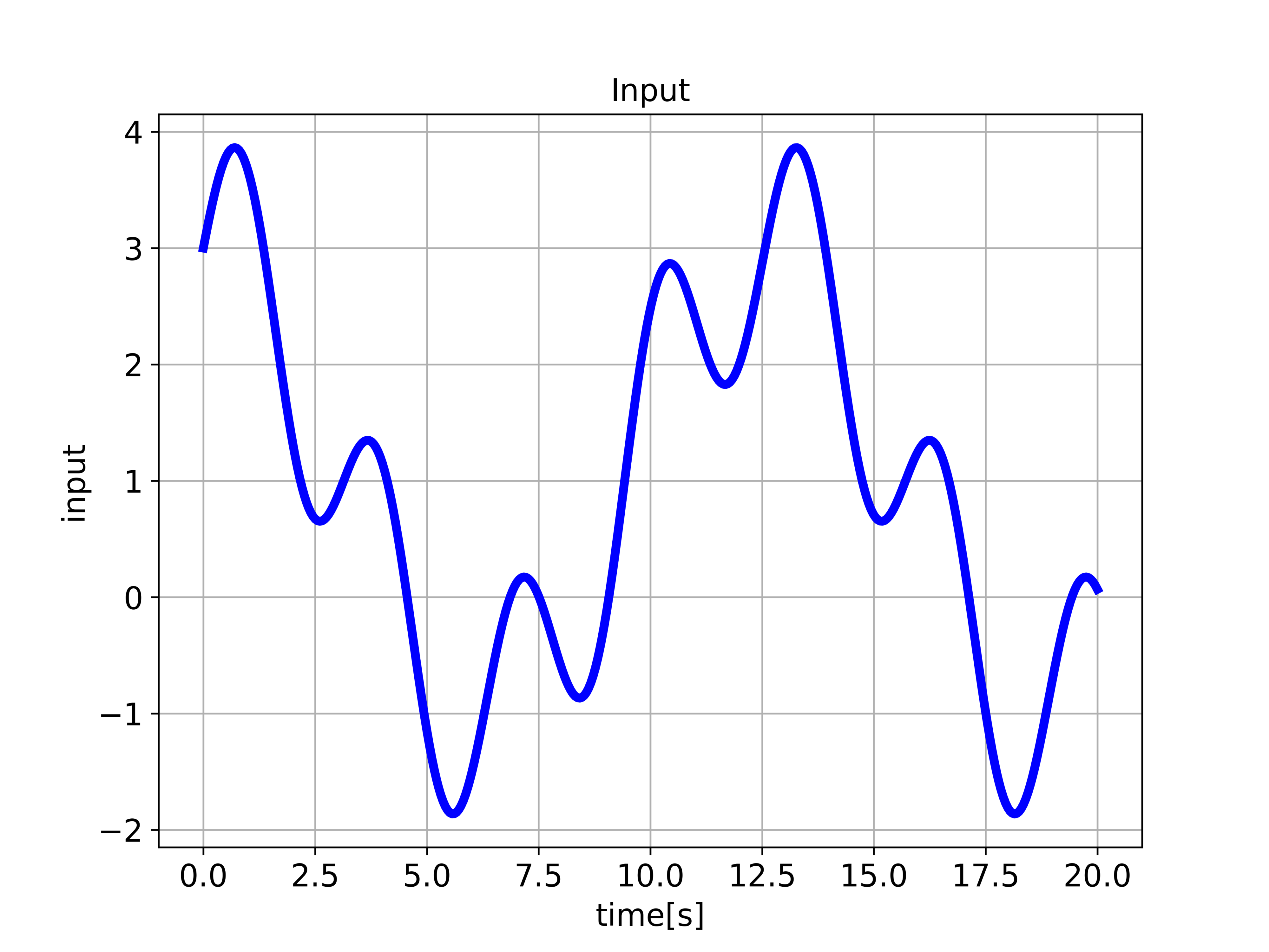
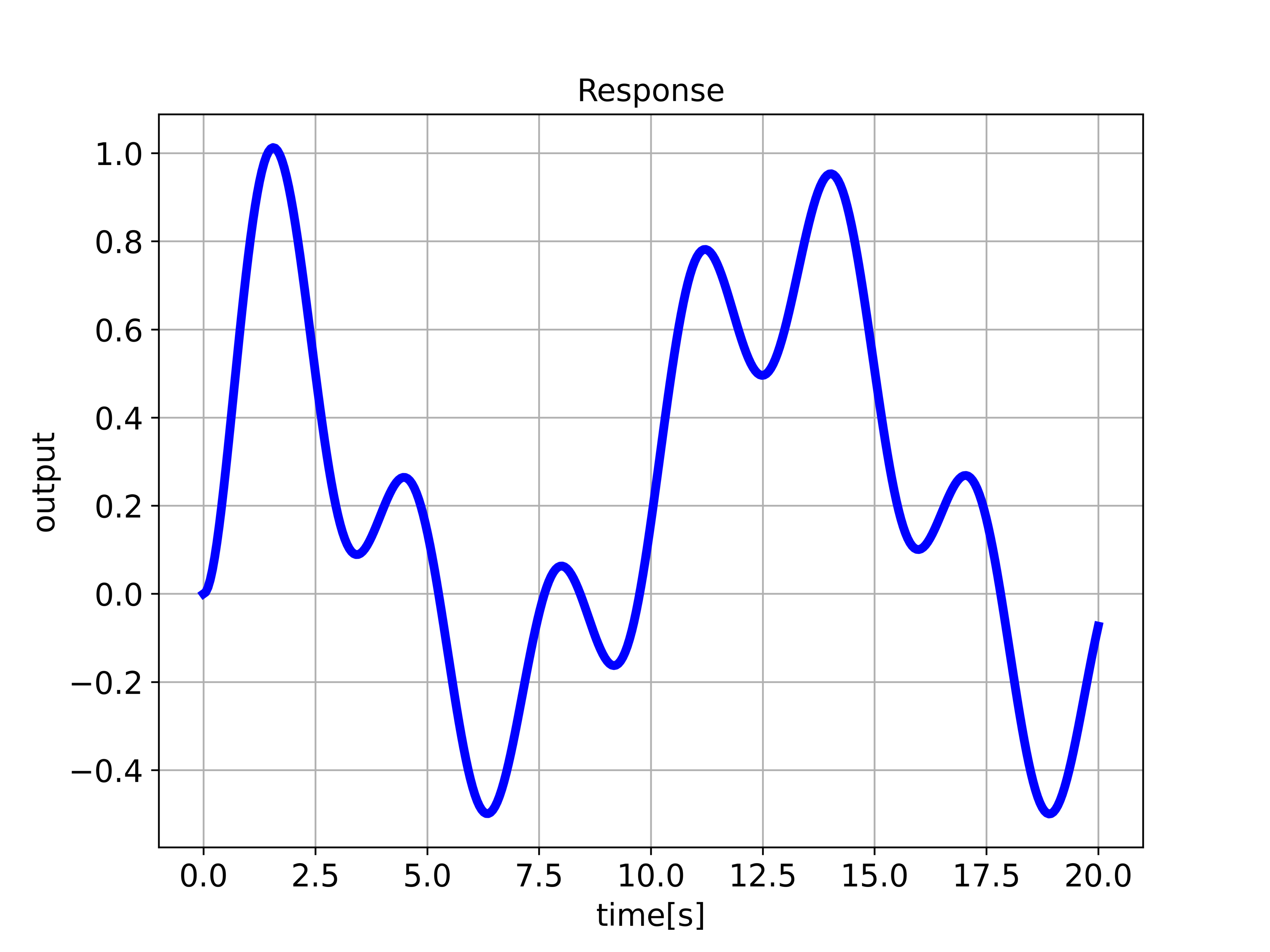
To simulate the response of a state-space model to user-defined input, we first need to define a time vector used for simulation. Then, we need to define the input. After that, we need to define the initial state and we need to use the function “ct.forced_response()” to compute the response for the user-defined input. The first input parameter is the state-space model object, and the second input parameter is the time vector. The third input parameter is the user-defined input. The function “ct.forced_response()” returns the time vector used for simulation and the computed response. The code given below computes and plots the input and simulated response.

timeVector2=np.linspace(0,20,400)

inputVector2=np.sin(2*timeVector2)+2*np.cos(0.5*timeVector2)+np.ones(timeVector2.shape)


plottingFunction(timeVector2,inputVector2,'Input',
                     'time[s]','input','input.png')


x0=np.array([[0],[0]])


timeReturned2, systemOutput2 =ct.forced_response(sysState,timeVector2,inputVector2)



plottingFunction(timeReturned2,systemOutput2,'Response',
                     'time[s]','output','forcedResponse.png')

The input used for the simulation is given below.

The simulated output is given below.

Obtain Information About Rise Time, Settling Time, Overshoot and Peak Value of Step Response in Python

To obtain information about rise time, settling time, overshoot and peak value of step response in Python, we use the function “ct.step_info”. The code and results are given below

stepInfoData=ct.step_info(sysState)

{'RiseTime': np.float64(0.8373036701796529),
 'SettlingTime': np.float64(4.046967739201656),
 'SettlingMin': np.float64(0.23487229056187936),
 'SettlingMax': np.float64(0.290758373226049),
 'Overshoot': np.float64(16.30334929041961),
 'Undershoot': 0,
 'Peak': np.float64(0.290758373226049),
 'PeakTime': np.float64(1.8141579520559146),
 'SteadyStateValue': np.float64(0.25)}

Poles, Zeros, and Damping Ratio of State-Space Model in Python

To compute poles, zeros, and damping ratio of state-space models in Python, we use this code

ct.damp(sysState,doprint=True)


ct.poles(sysState)


ct.zeros(sysState)

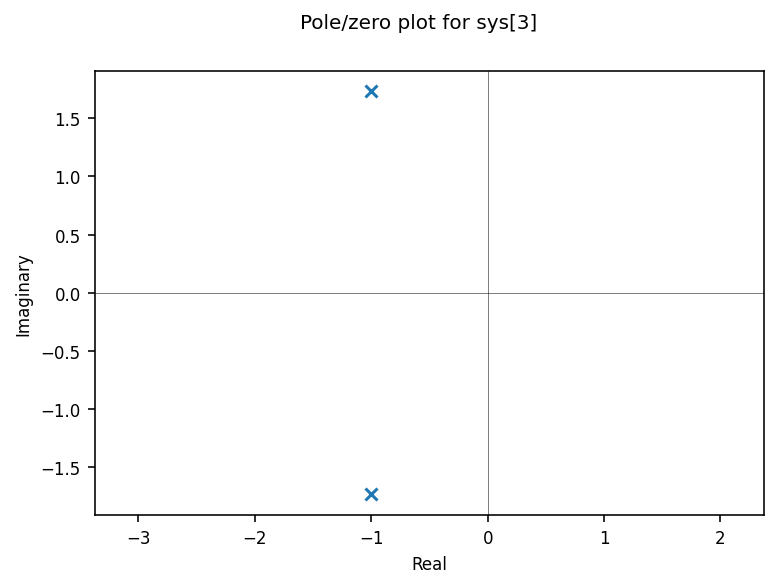
The pole-zero map can be plotted by using the function “ct.pzmap()”

ct.pzmap(sysState)

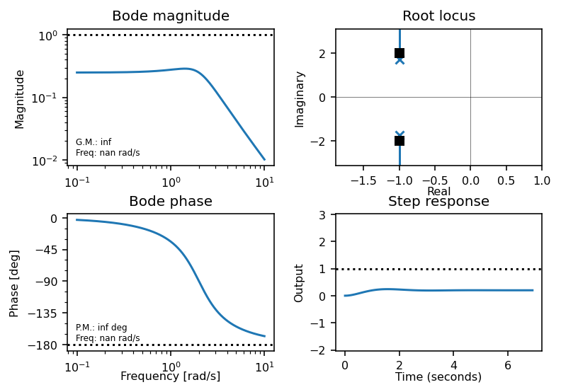
Bode, root-locus, and step response plots can be obtained on a single group by using “ct.sisotool()”

How to Discretize a State-Space Model in Python

To discretize the state-space model, we use the code given below

sampleTime=0.1

sysStateDiscrete=ct.sample_system(sysState,sampleTime, method='zoh')


sysStateDiscrete.A

sysStateDiscrete.B

sysStateDiscrete.C

sysStateDiscrete.D


sysStateDiscrete.isdtime()

We first need to specify the sampling time. To discretize, we use the function “ct.sample_system()”. The last input parameter is the discretization method. If you specify method =’zoh’, then the zero-order-hold method will be used. On the other hand, if you specify method=’bilinear’ a bilinear discretization method will be used. The discretized matrices can be obtained as follows

sysStateDiscrete.A

sysStateDiscrete.B

sysStateDiscrete.C

sysStateDiscrete.D