Introduction to Rotation Matrices in Robotics and Aerospace Engineering – Fusion of Engineering, Control, Coding, Machine Learning, and Science

In this tutorial, we provide a concise introduction to rotation matrices in robotics and aerospace engineering. We explain how to derive the rotation matrices for the 2D case. Everything explained in this tutorial can easily be generalized to the three-dimensional case. The YouTube tutorial accompanying this webpage is given below.

Problem Formulation

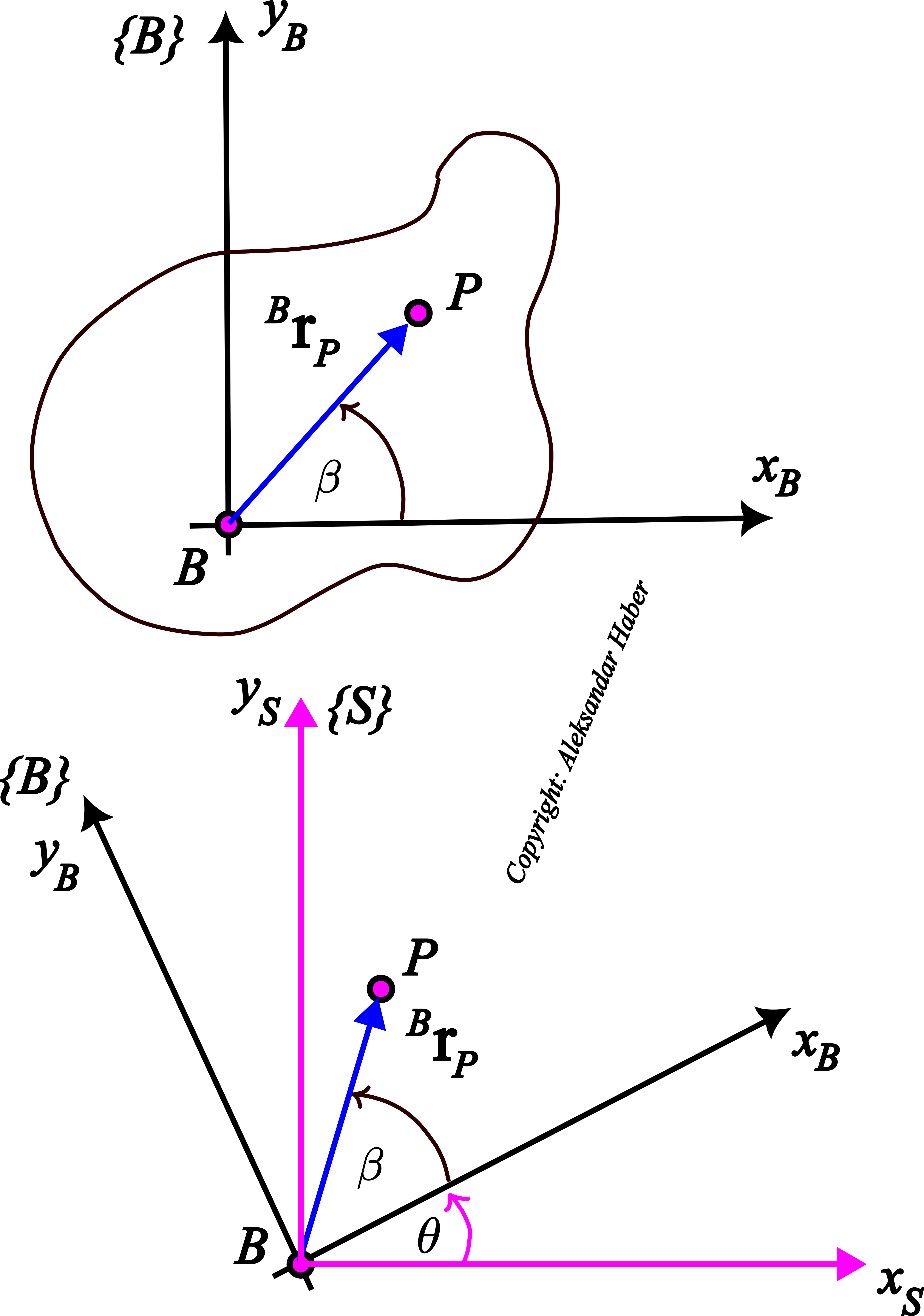
First, let us start with the problem formulation. We consider the figure shown below.

Figure 1: Rotation of the body frame $\{B \}$ with respect to the inertial frame $\{S \}$ .

The top panel of the figure shows a body frame $\{B\}$ and the point $P$ in that body frame. The point $P$ is a point of a body that can rotate around the point $B$ . The vector ${}^{B}\mathbf{r}_{P}$ is the distance vector of the point $P$ from the origin $B$ . The left superscript in the notation ${}^{B}\mathbf{r}_{P}$ means that the projections of the distance vector are expressed in the coordinate frame $\{B\}$ (see Fig. 2 below):

(1) $\begin{align*}{}^{B}\mathbf{r}_{P}=\begin{bmatrix} x_{BP} \\ y_{BP} \end{bmatrix}\end{align*}$

Since the point $P$ is a fixed point, the vector ${}^{B}\mathbf{r}_{P}$ rotates together with the body and the coordinate frame $\{B\}$ .

Next, we rotate the body for the angle of $\theta$ . The bottom panel of Fig. 1 above shows the situation after the rotation. The frame $\{B\}$ and the vector ${}^{B}\mathbf{r}_{P}$ are rotated for the angle of $\theta$ with respect to the frame $\{S \}$ . The frame $\{S \}$ denoted by the magenta color is fixed and it does not rotate. The frame $\{S \}$ is the inertial or the fixed frame.

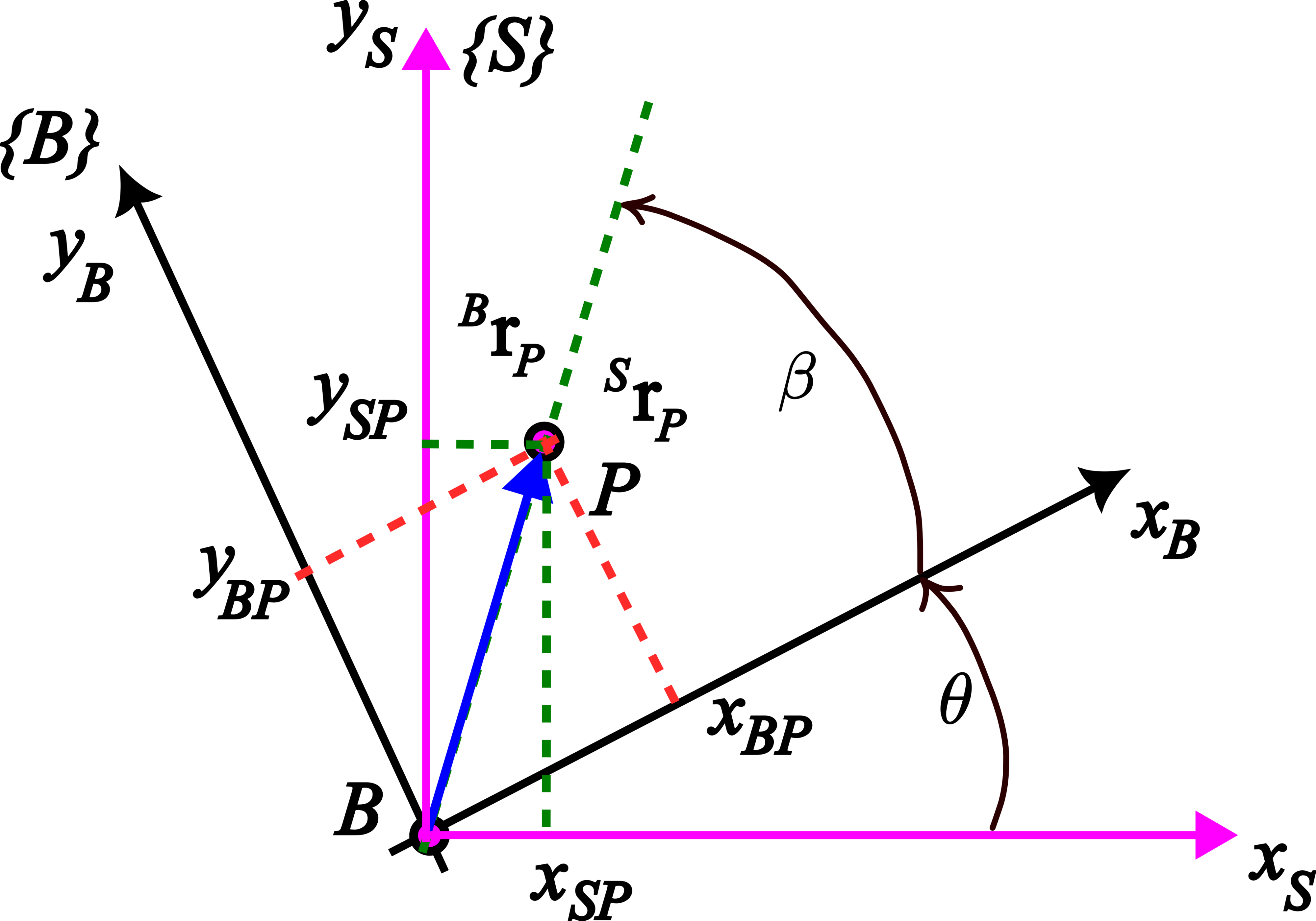
The next figure shows projections of the vector ${}^{B}\mathbf{r}_{P}$ in the frames $\{B \}$ and $\{S \}$ :

Figure 2: Projections of the distance vector $\mathbf{r}_{P}$ in the frames $\{B\}$ and $\{S\}$ .

The position vector $\mathbf{r}_{P}$ has two representations:

The representation of the position vector $\mathbf{r}_{P}$ in the frame $\{B\}$ :
(2) $\begin{align*}{}^{B}\mathbf{r}_{P}=\begin{bmatrix} x_{BP} \\ y_{BP} \end{bmatrix}\end{align*}$

where $x_{BP}$ and $y_{BP}$ are the projections of the distance vector $\mathbf{r}_{P}$ onto the axes of the frame $\{B\}$ .
The representation of the position vector $\mathbf{r}_{P}$ in the frame $\{S\}$ :
(3) $\begin{align*}{}^{S}\mathbf{r}_{P}=\begin{bmatrix} x_{SP} \\ y_{SP} \end{bmatrix}\end{align*}$

where $x_{SP}$ and $y_{SP}$ are the projections of the distance vector $\mathbf{r}_{P}$ onto the axes of the frame $\{S\}$ .

Problem formulation: Given the projections of the vector ${}^{B}\mathbf{r}_{P}$ in the frame $\{B \}$ , and the angle of rotation $\theta$ , compute the projections of the vector ${}^{S}\mathbf{r}_{P}$ in the frame $\{ S\}$ .

This problem is solved by deriving a rotation matrix. The rotation matrix will be used to transform the projections of the distance vector from one coordinate frame to another.

Derivation of the Rotation Matrix and Solution of the Projection Transform Problem

For presentation clarity and to simplify the notation, let us first denote the intensity of the vector ${}^{B}\mathbf{r}_{P}$ by $r$ . That is,

(4) $\begin{align*}r=|{}^{B}\mathbf{r}_{P} |\end{align*}$

From the above figure, we have:

(5) $\begin{align*}x_{SP}& =r\cos(\theta+\beta) \\y_{SP}& =r\sin(\theta+\beta)\end{align*}$

where $\beta$ is the angle that the vector ${}^{B}\mathbf{r}_{P}$ creates with the axis $x_{B}$ . Next, let us recall the basic formulas for the cosine and sine of two angles:

(6) $\begin{align*}\cos (\theta+\beta) =\cos (\theta) \cos (\beta) -\sin (\theta) \sin (\beta) \\\sin (\theta+\beta) =\sin (\theta) \cos(\beta)+\cos (\theta) \sin(\beta)\end{align*}$

By substituting these formulas in (5), we obtain

(7) $\begin{align*}x_{SP}& =r\cos(\theta+\beta)=r\cos (\theta) \cos (\beta) -r\sin (\theta) \sin (\beta) \\y_{SP}& =r\sin(\theta+\beta)=r\sin (\theta) \cos(\beta)+r\cos (\theta) \sin(\beta)\end{align*}$

Next, from Fig.2, it follows

(8) $\begin{align*}x_{BP}& =r\cos (\beta) \\y_{BP}& =r \sin(\beta)\end{align*}$

By substituting (8) in (7), we obtain

(9) $\begin{align*}x_{SP}& = \cos (\theta)x_{BP} -\sin (\theta) y_{BP} \\y_{SP}& =\sin (\theta) x_{BP}+ \cos (\theta) y_{BP} \end{align*}$

The last equation can be written in the matrix format

(10) $\begin{align*}\begin{bmatrix}x_{SP} \\y_{SP}\end{bmatrix} = \begin{bmatrix} \cos (\theta) & - \sin (\theta) \\ \sin (\theta) & \cos (\theta) \end{bmatrix}\begin{bmatrix} x_{BP} \\ y_{BP} \end{bmatrix}\end{align*}$

The last equation can be written compactly like this

(11) $\begin{align*}{}^{S}\mathbf{r}_{P} = {}^{S}_{B}R(\theta){}^{B}\mathbf{r}_{P}\end{align*}$

where

(12) $\begin{align*}{}^{S}\mathbf{r}_{P}=\begin{bmatrix}x_{SP} \\y_{SP}\end{bmatrix}, \; {}^{B}\mathbf{r}_{P}=\begin{bmatrix} x_{BP} \\ y_{BP} \end{bmatrix}, \; {}^{S}_{B}R(\theta)=\begin{bmatrix} \cos (\theta) & - \sin (\theta) \\ \sin (\theta) & \cos (\theta) \end{bmatrix}\end{align*}$

The matrix

(13) $\begin{align*}{}^{S}_{B}R(\theta)=\begin{bmatrix} \cos (\theta) & - \sin (\theta) \\ \sin (\theta) & \cos (\theta) \end{bmatrix}\end{align*}$

is called the rotation matrix. It transforms projections from the rotated frame $\{B \}$ to the frame $\{S \}$ . The subscript and superscript notation should be interpreted like that. The left superscript is the output frame and the left subscript is the input frame of the transformation.

The equation enables us to transform projections of a vector between two coordinate frames that are rotated with respect to one another.

Problem Formulation

Derivation of the Rotation Matrix and Solution of the Projection Transform Problem

admin

You might also like

How to Move and Jog an ABB Robot Using FlexPendant (Teach Pendant) – ABB Robotics Tutorial

How to Establish Serial Communication Between Python and Arduino in Linux Ubuntu

How to Memorize Robot Points using FlexPendant-Teach Pendant for ABB Robot Programming-ABB Tutorials