Introduction to (Direct) Lyapunov Stability Analysis With Examples

In this control engineering and control theory tutorial, we provide a brief introduction to Lyapunov stability analysis. The YouTube tutorial accompanying this tutorial is given below.

Motivation for Lyapunov Stability Analysis

Consider the following nonlinear dynamics

(1)  

where is a state vector, and is a (nonlinear) vector function. Let be an equilibrium point of (1). Here for simplicity, we assumed that 0 is an equilibrium point. However, everything stated in this tutorial can be generalized to the case of non-zero equilibrium points. This can be achieved with a simple change of state-space variables.

We want to provide answers to the following questions

1. Is the equilibrium point stable?
2. Is the equilibrium point asymptotically stable?

In the case of linear systems, these questions can easily be answered by computing the eigenvalues of the linear system. However, in the case of nonlinear systems, these questions are far from trivial.

There are at least two methods that we can use to answer these questions:

1. Lyapunov’s indirect method (also known as Lyapunov’s first method). The main idea of this approach is to linearize the dynamics of the nonlinear system around the equilibrium point and to investigate the stability of the linearized dynamics. If the linearized dynamics is asymptotically stable, then the equilibrium point of the nonlinear system is also asymptotically stable. If the linearized dynamics is not stable, then the equilibrium point of the nonlinear system is also not stable.
2. Lyapunov’s direct method (also known as Lyapunov’s second method). This approach is based on finding a scalar function of a state that satisfies certain properties. Namely, this function has to be continuously differentiable and positive definite. If the first derivative of this function with respect to time is negative semidefinite along the state trajectories, then we can conclude that the equilibrium point is stable. On the other hand, if the first derivative along state trajectories is negative definite then the equilibrium point is asymptotically stable.

This tutorial is dedicated to the practical application of Lyapunov’s direct method. Before reading this tutorial it is a very good idea to revise the concept of positive (negative) definite functions. These concepts are explained in our previous tutorial, which can be found here.

Formal Statment of the Lyapunov Theorem for the Local Stability of Equilibrium Point

Before we introduce examples, it is very important to state the Lyapunov local stability theorem for an equilibrium point of a dynamical system. This theorem is stated in a number of standard textbooks on nonlinear systems, such as:

1. Nonlinear Systems, by Hassan K. Khalil (edition from 1992, page 101.)
2. Applied Nonlinear Control, by Jean-Jacques E. Slotine and Weiping Li (edition from 1991, page 62.)

Lyapunov (local) Stability Theorem: Consider a dynamical system

(2)  

where is a state vector, and is a (nonlinear) vector function. Let be an equilibrium point of (2). Let us assume that we are able to find a continuously differentiable scalar function of the state vector argument , defined on a neighborhood set of , that satisfies the following two conditions:

1. The function is (locally) positive definite in . That is, and in for all in .
2. The time derivative of along state trajectories of the system is (locally) negative semi-definite in . That is, for all in .

Then, is stable.

In addition, if the first time derivative of is (locally) negative definite in along any state trajectory of the system. That is, in , then is asymptotically stable.

In this brief tutorial, we give an intuitive explanation of Lyapunov’s stability theorem for one-dimensional system. This example is also explained in the accompanying video tutorial.

A positive definite function is shown below.

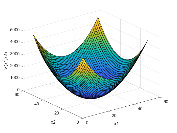
The function that satisfied the conditions of this theorem is called the Lyapunov function.

First Example of Stability Analysis

We consider the pendulum system shown in the figure below.

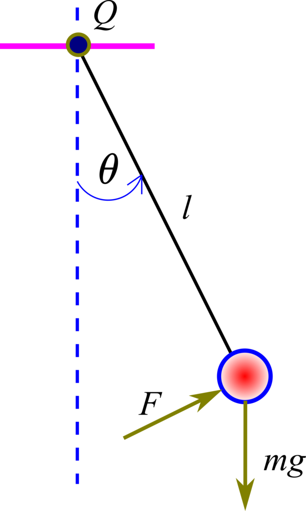
In this figure, is the rotation angle, is the length of the rod, is the mass of the ball, is the gravitational acceleration constant, and is the control force (external input). In our previous tutorial, which can be found here, we derived the equation of motion of this system. The equation has the following form

(3)  

For stability analysis, we always assume that the control force is equal to zero. That is, we study the dynamical behavior of the system without any external control actions. Under this assumption, the dynamics is given by the following equation

(4)  

Next, let us transform this equation into the state-space form by assigning the state variables

(5)  

The state-space model has the following form

(6)  

Next, let us simulate the state trajectories of such a system. In our previous tutorial, which can be found here, we explained how to simulate state trajectories in MATLAB. By entering the system dynamics (6) in the developed MATLAB codes, we obtain a phase portrait of the system. The phase portrait is given below. It is generated for the initial conditions and .

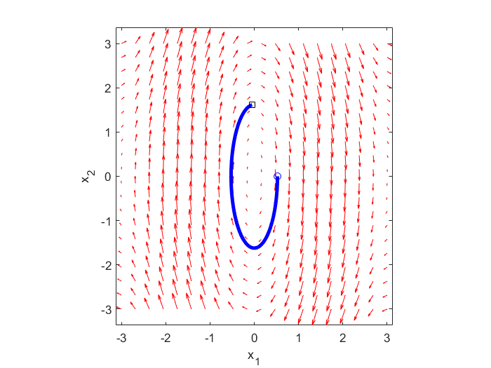
As can be observed from the figure above, the equilibrium point is stable, however, it is NOT asymptotically stable.

Let us now construct a Lyapunov function that will be used to formally prove that the equilibrium point is asymptotically stable. For that purpose, let us consider the figure shown below

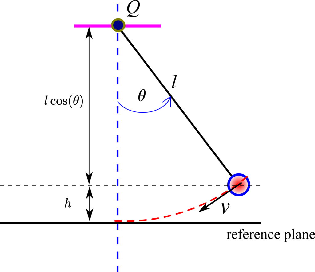
A good initial choice of the Lyapunov function is the total energy of the system. This is because if the system is asymptotically stable, then the energy of the system should decrease over time or if the system is stable, then the total energy is either constant or bounded (not increasing). Consequently, let us define the total energy of the system. The total energy is a sum of potential and kinetic energy:

(7)  

where is the velocity of the mass, and is the distance of the mass from the reference plane for calculating the potential energy. Since and , the total energy becomes:

(8)  

This function should be positive definite and . Since and the kinetic energy is zero for , it is obvious that . Then, let us investigate the positive definiteness of this function. Obviously, the kinetic energy is always positive for . Then, the potential energy is always positive for , for . Consequently, we conclude that the function (8) is positive definite over the domain defined by

(9)  

Next, let us compute the derivative of the function along the state trajectories of the system:

(10)  

Next, we substitute and from (6) in (10). As the result, we obtain

(11)  

Consequently, according to the Lyapunov local stability theorem, the equilibrium point is stable.

The physical interpretation of this result is that the energy stays constant along the trajectories of the system! This is actually the law of energy conservation. That is, the potential energy transforms into the kinetic energy and vice-versa. However, the total energy remains constant!