In this tutorial, we provide a clear and correct explanation of the linearization of dynamical systems. The motivation for creating this tutorial comes from the fact that online we can find a number of tutorials that do not correctly or clearly explain the linearization process of dynamical systems. Consequently, this tutorial aims to provide a clear, concise, and correct explanation of the linearization process. The YouTube tutorial accompanying this post is given below.

Motivational example
We consider a simple gravity pendulum shown in the figure below.

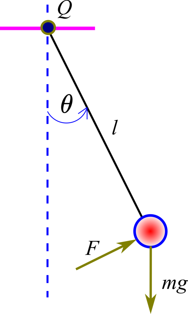
A ball (red color in the figure) with a mass of 


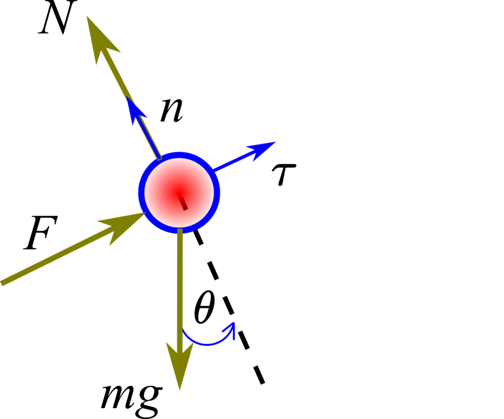
In the figure above, 


(1) 

where 


(2) 

On the other hand, the tangential acceleration is given by
(3) 

where 


(4) 

From this equation, we obtain
(5) 

For simplicity, we assume that the control force
(6) 

where 
(7) 

Obviously, this system is nonlinear since
- It nonlinearly depends on the dependent variable
- It nonlinearly depends on the input
Let us write the ordinary differential equation (7) in the state-space form. First, we introduce the state-space variables
(8) 

By differentiating the last two equations, we obtain
(9) 

Consequently, the state-space model has the following form
(10) 

Usually, we compactly write this state-space model as follows
(11) 

where 


(12) 

In our case, we have
(13) 

Later in this tutorial, we will get back to our nonlinear model. Next, we explain the linearization process.
Linearization Procedure
Consider the figure shown below.

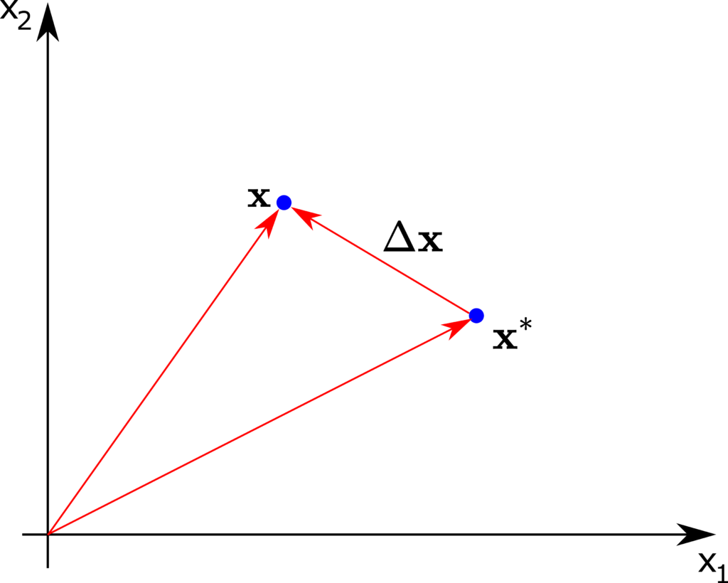
The quantities in this figure are


(14)


The vector
(15) 

Where 

When linearizing the dynamics, we have the freedom of choice to choose the vector
- The equilibrium point of the system. That is, the equilibrium point
(16)

Note here, that the equilibrium points are computed for
- The steady state of the system. Let us assume that there is a constant input vector
(17)

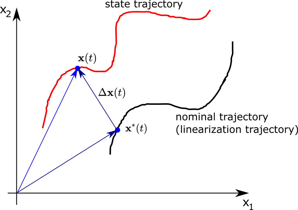
since both - The nominal trajectory. Instead of selecting the linearization state vector as a steady-state vector or an equilibrium point, the state vector can be selected as a point on a state trajectory. In this case, we have
(18)

For a known
(19)

The solution


Besides these selections, we can also approximate the dynamics around other states and inputs.
The general idea of Linearization
First, let us recall the linearization procedure of nonlinear algebraic functions. Consider the following scalar function 


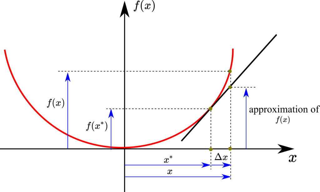
Let us assume that we want to approximate the function 
(20) 

The right-hand side of the last equation is an equation of a tangent line through the point 
(21) 

Let us consider the following example
(22) 

Let us approximate this function at the point 
(23) 

The linearization of nonlinear state-space models is similar in spirit to the linearization of scalar nonlinear functions. In the sequel, we explain the linearization procedure of state-space models.
We approximate the nonlinear function 


(24) 

where
(25) 

and where
(26) 

The vertical lines in (24) mean that the matrices are evaluated at the points
(27) 

On the other hand, from (25), we obtain
(28) 

Consequently, from (27) and (28), we obtain
(29) 

By replacing the approximation with equality, we obtain
(30) 
Let us introduce a new notation
(31) 

From (30) and (31), we obtain the linearized model
(32) 

where
- The system matrices


(33) 

- The linearized state vector and linearized input vector are defined by
(34) 

It should be kept in mind that the linearization produces a reliable approximation of the nonlinear system only for relatively small values of 

Linearization of Nonlinear Pendulum Equations
The nonlinear state-space model is given by the following equation
(35) 
From this equation, we obtain
(36) 

The Jacobian matrix with respect to the state is defined by
(37) 

The Jacobian matrix with respect to the control input is defined by
(38) 

We approximate the nonlinear system at the state and input
(39) 

For this selection of the state and input, we obtain
(40) 

The final linearized model is given by
(41) 
