Plot Phase Portraits and State-Space Trajectories of Dynamical Systems in MATLAB

In this tutorial, we explain how to generate phase portraits and state-space trajectories of dynamical systems in MATLAB. The YouTube video accompanying this post is given below. The GitHub page with all the codes is given here. Besides this tutorial, we created a tutorial on how to generate phase plots of dynamical systems in Python. The Python tutorial is given here.

For example, consider the following dynamical system:

(1)  

In this tutorial, you will learn how to generate a phase portrait of this system. The phase portrait is shown in the figure below.

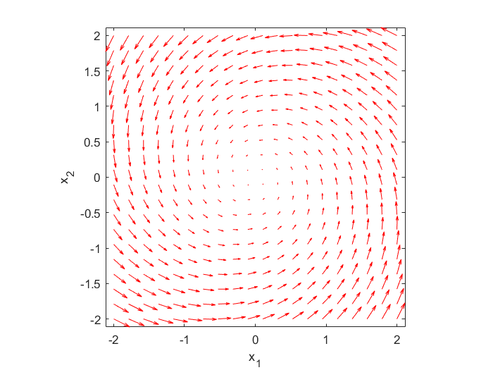
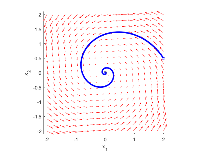
Also, you will learn how to plot a particular state-space trajectory obtaining by simulating (1) from a given initial condition. A simulated state trajectory (blue line) is shown in Figure 2 below.

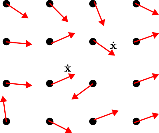
The basic idea for drawing the phase portraits is illustrated in Fig. 3. and Fig. 4.

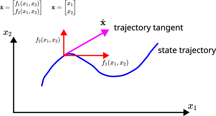
Consider the general form of a state-space model of a dynamical system:

(2)  

The vector defines a tangent to the state-space trajectory shown in Fig. 1. The components of the tangent vector are and . Consequently, for known values of and we can construct the tangent vector . The tangent vectors at trajectory points define the phase portraits. Consequently, to construct the phase portrait, we construct a grid shown in Fig. 4. Then, at every point of this grid, we calculate the tangent vector. These tangent vectors define the phase portrait.

In the sequel, we explain how to generate phase portraits and state-space trajectories in MATLAB. The first step is to define a MATLAB function that describes the dynamics of the system (1). This function is given below.

% define the nonlinear, continious-time, state-space model
% t is time
% x is the vector of state coordinates
% Author: Aleksandar Haber
% Date: December 2022
function dx = dynamics(t,x)
%dx=[x(2); -sin(x(1));];
%dx=[-2*x(1);-3*x(2)];
dx=[-1*x(1)-3*x(2);3*x(1)-1*x(2)];
end

This function should be saved as “dynamics.m” since it will be called from other functions. The function takes time and state vector as an argument, and it computes the right-hand side of (1). That is, it computes for given . Notice that we commented code lines defining two different forms of the dynamics. You can uncomment these lines and comment the other ones in order to generate the phase portrait of other systems.

Next, we define the function that actually plots the phase portrait. This function is given below.

% Function that sketches a phase portrait of a dynamical system
% Author: Aleksandar Haber, December 2022

% f is a function that defines the nonlinear state-space model
% this function should be defined in an external file

% vectors x1 and x2 define the coordinates of points
% in a rectangular region that is defined by the meshgrid function
function phase_portrait(f,x1,x2)
[x,y] = meshgrid(x1,x2);
u = zeros(size(x));
v = zeros(size(x));
% we can use a single loop over each element to compute the derivatives at each point 
t=0; 
% we want the derivatives at each point at t=0, i.e. the starting time
[d1,d2]=size(x);

for i = 1:d1
    for j=1:d2
    Yprime = f(t,[x(i,j); y(i,j)]);
    u(i,j) = Yprime(1);
    v(i,j) = Yprime(2);
    end
end


% for i = 1:d1
%     for j=1:d2
%             Vmod = sqrt(u(i,j)^2 + v(i,j)^2);
%             u(i,j) = u(i,j)/Vmod;
%             v(i,j) = v(i,j)/Vmod;
%     end
% end

figure(1)
hold on
% quiver(X,Y,U,V) plots velocity vectors as arrows with components (u,v) at the points (x,y)
quiver(x,y,u,v,'r'); 
xlabel('x_{1}')
ylabel('x_{2}')
axis tight equal;
box
end

This function should be saved as “phase_portrait.m”. The first argument of this function is a MATLAB function handle that defines the system dynamics. In our case the dynamics is defined in the file “dynamics.m”. Consequently, a handle to this function will be passed as the first argument to “phase_portrait.m”. The second and third arguments are vectors that represent the and points that will be used to plot phase portraits. The code lines

[x,y] = meshgrid(x1,x2);
u = zeros(size(x));
v = zeros(size(x));

are used to generate the meshgrid matrices x and y. Also, these code lines are used to define empty matrices u and v. These matrices are used to store and , respectively, computed at the meshgrid points that are defined by the matrices x and y. An explanation of the meshgrid function is given in our previous tutorial which can be found here. The matrices u and v are populated by using this piece of code

for i = 1:d1
    for j=1:d2
    Yprime = f(t,[x(i,j); y(i,j)]);
    u(i,j) = Yprime(1);
    v(i,j) = Yprime(2);
    end
end

Basically, we compute the right-hand side of (1) for meshgrid points defined by the matrices x and y. This is done by calling the function f, which in our case is a function handle. We actually call the previously defined function . The matrix entry is identical to component of the tangent vector in Fig. 3. Similarly, the matrix entry is identical to component of the tangent vector in Fig. 3. That is and define the tangent vectors at meshgrid points. Once we populate the matrices u and v, we use the MATLAB function quiver() to plot the phase portrait. This function is used to plot velocity vectors. In our case, the velocity vectors are the tangent vectors .

The plotting function “phase_portrait” is called from our main code which is given below.

% Phase portraits of dynamical systems
% Author: Aleksandar Haber, 
% Date: December 2022
clear 
% time steps for control 
% First draw the phase portrait of the system 
x1=linspace(-2,2,20);
x2=linspace(-2,2,20);
phase_portrait(@dynamics,x1,x2)


% discretization steps
T=0.01; 
% check the discrete-time model vs. continious time model
time=[0:T:20];
initialState=[2;0.5];
% generate continious-time response
[ts,ys] = ode45(@dynamics,time,initialState);
hold on;
plot(ys(:,1),ys(:,2),'b','LineWidth',3)
plot(ys(1,1),ys(1,2),'bo') % starting point
plot(ys(end,1),ys(end,2),'ks') % ending point

First, we define two vectors and that define the limits of our phase space, resolution, as well as the meshgrid. Then, we simply call the function “phase_portrait” to plot the phase portrait. In the second part of the code (starting from the code line 12), we solve (integrate) the dynamics defined in the function “dynamics.m”. We use the standard MATLAB solver . More details about solving the dynamics in MATLAB are given in our previous post, which can be found here and here.

These code lines generate figures 1 and 2 given at the beginning of this post.