Extended Kalman Filter Tutorial With Example and Disciplined Python Codes – PART I -Derivation

In this tutorial, we derive the extended Kalman filter that is used for the state estimation of nonlinear systems. We furthermore develop a Python implementation of the Kalman filter and we test the extended Kalman filter by using an example of a nonlinear dynamical system. In this first part of the tutorial, we explain how to derive the extended Kalman filter.

The YouTube videos accompanying this tutorial are given below.

PART 1:

PART 2:

Before reading this tutorial, it is recommended to go over these tutorials on linear Kalman filtering:

1. Introduction to Kalman Filter: Derivation of the Recursive Least Squares Method
2. Introduction to Kalman Filter: Disciplined Python Implementation of Recursive Least Squares Method
3. Time Propagation of State Vector Expectation and State Covariance Matrix of Linear Dynamical Systems – Intro to Kalman Filtering
4. Kalman Filter Tutorial- Derivation of the Kalman Filter by Using the Recursive Least-Squares Method
5. Disciplined Kalman Filter Implementation in Python by Using Object-Oriented Approach
   

General Information About Extended Kalman Filter

The extended Kalman filter is a generalization of the linear Kalman filter for nonlinear dynamical systems in the fairly general mathematical form given by the following state and output equations:

(1)  

where

• is a discrete-time instant. That is, we look at the system behavior at the time instants , where is the sampling period of the system. That is, before applying the filter, we assume that the signals are sampled in time.
• is the -dimensional state vector at the discrete-time instant .
• is the -dimensional input vector at the discrete-time instant .
• is the -dimensional disturbance vector affecting the state and dynamics of the system. This vector is also called the process noise vector. We assume that the disturbance vector is white, zero-mean, uncorrelated, with the covariance matrix given by .
• is the -dimensional output vector. This vector is also known as the observation vector.
• is the -dimensional measurement noise vector. We assume that the measurement noise vector is white, zero-mean, uncorrelated, with the covariance matrix given by .
• is the nonlinear vector function that is allowed to vary from one time instant to another. This functions mathematically models the dynamics of the system.
• is the nonlinear vector function that is allowed to vary from one time instant to another. This function mathematically models the relationship between the observed vector and the state of the system.

Before we start with the development of the extended Kalman filter, we need to explain the following notation. In Kalman filtering, we have two important state estimates: the a priori state estimate and the a posteriori state estimate. Apart from this post and Kalman filtering, a priori and a posteriori are Latin phrases whose meaning is explained here.

The a priori state estimate of the state vector is obtained implicitly on the basis of the output vector measurements (as well as on some other information that will be explained later). That is, the a priori state estimate is obtained on the basis of the past measurements up to the current discrete-time instant and NOT on the basis of the measurement at the current discrete-time instant . The a priori state estimate is denoted by

(2)  

where “the hat notation” denotes an estimate, and where the minus superscript denotes the a priori state estimate. The minus superscript originates from the fact that this estimate is obtained before we process the measurement at the time instant .

The a posteriori estimate of the state is obtained implicitly on the basis of the measurements . The a posteriori estimate is denoted by

(3)  

where the plus superscript in the state estimate notation denotes the fact that the a posteriori estimate is obtained by processing the measurement obtained at the time instant .

Another concept that is important for understanding and implementing the extended Kalman filter is the concept of the covariance matrices of the estimation error. The a priori covariance matrix of the state estimation error is defined by

(4)  

On the other hand, the a posteriori covariance matrix of the state estimation error is defined by

(5)  

Derivation of the Extended Kalman Filter

We start from the nonlinear state equation that is rewritten over here for clarity

(6)  

Let us assume that at the discrete-time instant the a posteriori estimate is available. Also, let us assume that the value of is also known at this time instant. The first main idea of the extended Kalman filter is to linearize the state equation around . So, let us do that. By linearizing the state equation, we obtain

(7)  

where

• The matrix is obtained by linearizing the nonlinear dynamics around and

(8)  

where is the known value of the input at the time instant . This matrix is the Jacobian matrix of the function evaluated at and . The Jacobian matrix is defined by

(9)  

where

(10)  

That is, the th entry of the Jacobian matrix is the partial derivative of the th entry of the vector function with respect to the th entry of the state vector .

• The vector contains known quantities at the time instant and is defined as

(11)  

The next step is to linearize the output equation. As it will be explained later, at the time instant we can propagate the state estimate through the nonlinear dynamics to compute . We do that before the output measurement at the time instant arrives. The second main idea of the Kalman filter is to linearize the output equation around the known value of the a priori state estimate . Let us do that. First, for clarity, here is our output equation again:

(12)  

The linearization procedure produces:

(13)  

where

• The matrix is obtained by linearizing the nonlinear output equation around

(14)  

This matrix is the Jacobian matrix of the function evaluated at . The Jacobian matrix is defined by

(15)  

where

(16)  

That is, the th entry of the Jacobian matrix is the partial derivative of the th entry of the vector function with respect to the th entry of the state vector .

The vector is defined as follows

(17)  

It is important to emphasize that this vector is completely known.

Let us now summarize the linearized state and output equations:

(18)  

The third main idea of the extended Kalman filter is to apply the linear Kalman filter to these equations. The only divergence from the linear Kalman filter is to use the nonlinear state equation to propagate the a posteriori estimates in time. We derived the linear Kalman filter in our previous tutorial which can be found here. Consequently, we will use the derived equations and apply them to our case.

EXTENDED KALMAN FILTER:

At the initial discrete-time step we select an initial a posteriori estimate and an initial a posteriori covariance matrix of the estimation error . Then, for we recursively perform the following steps:

STEP 1 (after the time step and before the time step ): At this time step we know the a posteriori estimate and the a posteriori covariance matrix from the time step . First, we compute the linearized matrix :

(19)  

Then, we compute the a priori estimate and the a priori covariance matrix for the upcoming time step by propagating and through the nonlinear dynamics and the covariance equation

(20)  

At the end of this step, compute the Jacobian matrix of the output equation

(21)  

STEP 2 (immediately after the time step ): At the time step , the measurement arrives. Immediately after the time step , we compute the Kalman gain matrix

(22)  

Then, compute the a posteriori state estimate:

(23)  

where the third form of the above-stated equation is the most appropriate for computations. Finally, compute the a posteriori covariance matrix by using either this equation

(24)  

or

(25)  

Due to numerical stability, the equation (25) is a more preferable option to be used for covariance matrix time propagation.

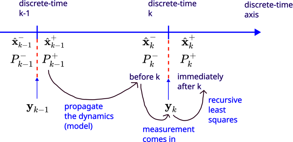
The above-summarized two steps are graphically illustrated in the figure below.