In this tutorial, we present a simple derivation of the Kalman filter equations. Before reading this tutorial, we advise you to read this tutorial on the recursive least squares method, and this tutorial on mean and covariance matrix propagation through the system dynamics. In the follow-up post which can be found here, we explain how to implement the Kalman filter in Python. The YouTube video accompanying this post is given below.

Model and Model Assumptions
We are considering the following state-space model of a dynamical system:
(1) 

where


![Q_{k}=E[\mathbf{w}_{k}\mathbf{w}_{k}^{T}]](https://aleksandarhaber.com/wp-content/ql-cache/quicklatex.com-266e7fa5fa9769934ad70b1a27d1a31b_l3.png "Rendered by QuickLaTeX.com")
![E[\cdot]](https://aleksandarhaber.com/wp-content/ql-cache/quicklatex.com-3941b329206b0baa01fad23b819cc5f7_l3.png "Rendered by QuickLaTeX.com")


![R_{k}=E[\mathbf{v}_{k}\mathbf{v}_{k}^{T}]](https://aleksandarhaber.com/wp-content/ql-cache/quicklatex.com-90d194c388d2c49758f447864c1e864d_l3.png "Rendered by QuickLaTeX.com")


This is a time-varying system. However, if the system is time-invariant, then all the system matrices are constant. We assume that the covariance matrices 


A priori and a posteriori state estimates, errors, and covariance matrices
In Kalman filtering, we have two important state estimates: a priori state estimates and a posteriori state estimates. Apart from this post and Kalman filtering, a priori and a posteriori are Latin phrases whose meaning is explained here.
The a priori state estimate of the state vector 


(2) 

where “the hat notation” denotes an estimate, and where the minus superscript denotes the a priori state estimate. The minus superscript originates from the fact that this estimate is obtained before we process the measurement
The a posteriori estimate of the state 

(3) 

where the plus superscript in the state estimate notation denotes the fact that the a posteriori estimate is obtained by processing the measurement
In our previous post, we explained how to derive a recursive least squares method from scratch. We defined and derived the expression for the covariance matrices of estimation errors in the context of recursive least squares filtering. Here, we also need to introduce covariance matrices of the a priori and a posteriori estimation errors. The covariance matrices of the a priori and a posteriori estimation errors are defined as follows
(4) ![\begin{align*}P_{k}^{-}=E[(\mathbf{x}_{k}-\mathbf{x}_{k}^{-})(\mathbf{x}_{k}-\mathbf{x}_{k}^{-})^{T}] \\P_{k}^{+}=E[(\mathbf{x}_{k}-\mathbf{x}_{k}^{+})(\mathbf{x}_{k}-\mathbf{x}_{k}^{+})^{T}]\end{align*}](https://aleksandarhaber.com/wp-content/ql-cache/quicklatex.com-2b8ca14220c48b39e392f9fa5c217e86_l3.png "Rendered by QuickLaTeX.com")

where 


Derivation of Kalman Equations from the Recursive-Least Squares Method
The following figure illustrates how the Kalman filter works in practice.

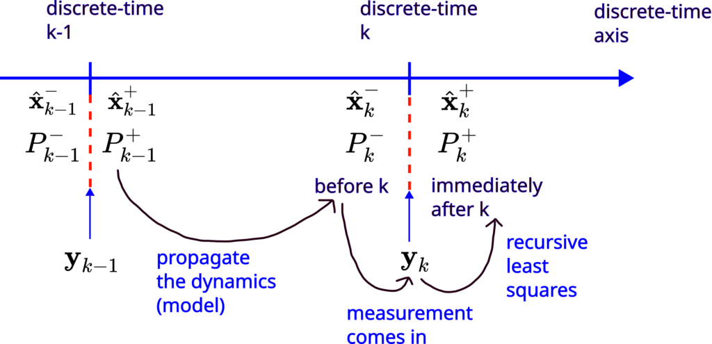
For the time being it is beneficial to briefly explain this figure. Even if some concepts are not completely clear, they will become clear by the end of this post. Immediately after the discrete-time instant 


Now that we have a general idea of how Kalman filtering works, let us now derive the Kalman filter equations. At the initial time instant 


(5) 

Then, the question is how to compute the a priori estimate 


The natural answer is that the system states, as well as the estimates, need to satisfy the system dynamics (1), and consequently,
(6) 

where we excluded the disturbance part since the disturbance vector is not known. Besides the initial guess of the estimate, we also need to select an initial guess of the covariance matrix of the estimation error. That is, we need to select 


(7) 

By using this expression, we obtain the following equation for
(8) 

So this is the best we can do at the initial time step 


At the time instant
To update these quantities, we need to use the recursive least-squares method. We derived the equations of the recursive least-squares method in our previous post, which can be found here. Here are the recursive least-squares equations:
- Update the gain matrix

(9)

- Update the estimate:
(10)

- Propagate the covariance matrix by using this equation:
(11)

or this equation(12)


Now, the question is how to use these equations to derive the Kalman filter equations? First, we perform the following substitutions in the recursive least-squares equations (these substitutions will be explained later in the text):
(13) 

(14) 

(15) 

(16) 

Here is the main idea behind these substitutions. Let us first focus on the equation (13). In the case of the recursive least squares method, the covariance before the measurement arrives is 


After these substitutions, we obtain the update equations:
(17) 

(18) 

(19) 

Now, let us go back at the time instant
(20) 

As the result, we obtained 


(21) 

to obtain 


- Before the measurement arrives, use the system dynamics to propagate the a posteriori estimate and covariance matrix of the estimation error from the step
- At the time step
This is illustrated in Fig. 2 (the same as Fig. 1 which is repeated here for completeness).

Let us now summarize the Kalman filter equations.
Summary of the derived Kalman filter equations
In the initial step, we select and initial estimate 


Step 1: Propagate the a posteriori estimate 
(22) 

Step 2: Obtain the measurement
(23) 

Here are a few comments about the derived Kalman filter equations. The matrix
(24) 

is more numerically stable and robust than the alternative equation
(25) 

Consequently, the equation (24) is preferable for computing the covariance update. Another important thing to mention is that the Kalman filter gain 


