Introduction to Kalman Filter: Disciplined Python Implementation of Recursive Least Squares Method

In our previous post which can be found here, we derived equations describing the recursive least-squares method. In this post, we explain how to implement the recursive least squares method in Python from scratch. We explain how to implement this method in a disciplined and clean manner, such that the developed code is modular and such that the code can easily be modified or used in other projects. This tutorial is important since it can serve as the basis for learning how to properly implement the Kalman filter in Python. Namely, as we have explained in our previous post, the Kalman filter equations are derived from the recursive least squares method. Consequently, it is important to first understand the Python implementation of the recursive least squares method. The GitHub page with all the codes is given here.

The YouTube video accompanying this post is given here:

As we have explained in our previous post, the recursive least squares method consists of the following three equations

1. Gain matrix update
   

   (1)  

2. Estimate update
   

   (2)  

3. Propagation of the estimation error covariance matrix by using this equation
   

   (3)  

   
   or this equation
   

   (4)  

   
   
   If no apriori knowledge of the estimate is known, then this method is initialized with the estimation error covariance matrix that is equal to , where is a large number, and with a random value of .

here

• is a discrete-time instant
• is the gain matrix
• is an estimate of the unknown variable
• is the measurement at the discrete-time instant ,
• is the measurement matrix of the measurement model
• is the measurement noise
• is the estimation error covariance matrix
• is the measurement noise covariance matrix
• is an identity matrix

It should be noted that this is a vector representation of the algorithm, that is, all the variables are vectors.

Our goal is to implement these equations. Our goal is to write a Python class that implements the recursive least squares method. This class should have a constructor that should initialize all the variables and create lists that will store the gain matrices, estimates, estimation errors, and estimation error covariance matrices. Also, this class should memorize the current time step . Also, this class should have a method (function) that should compute the above equations on the basis of the arrived measurement and update the lists that store the previous variables. Also, after the measurement arrives this method should update the current time step . Here, we should emphasize that we write a class that memorizes all the vectors and matrices from the beginning of the estimation process. This is done for diagnostic purposes. In practice, we do not need to do that, since we only need to memorize the variables from the previous time step .

The Python class implementing the recursive least squares method is given below

class RecursiveLeastSquares(object):
    
    # x0 - initial estimate used to initialize the estimator
    # P0 - initial estimation error covariance matrix
    # R  - covariance matrix of the measurement noise
    def __init__(self,x0,P0,R):
        
        # initialize the values
        self.x0=x0
        self.P0=P0
        self.R=R
        
        # this variable is used to track the current time step k of the estimator 
        # after every time step arrives, this variables increases for one 
        # in this way, we can track the number of variblaes
        self.currentTimeStep=0
                  
        # this list is used to store the estimates xk starting from the initial estimate 
        self.estimates=[]
        self.estimates.append(x0)
         
        # this list is used to store the estimation error covariance matrices Pk
        self.estimationErrorCovarianceMatrices=[]
        self.estimationErrorCovarianceMatrices.append(P0)
        
        # this list is used to store the gain matrices Kk
        self.gainMatrices=[]
         
        # this list is used to store estimation error vectors
        self.errors=[]
    
     
    # this function takes the current measurement and the current measurement matrix C
    # and computes the estimation error covariance matrix, updates the estimate, 
    # computes the gain matrix, and the estimation error
    # it fills the lists self.estimates, self.estimationErrorCovarianceMatrices, self.gainMatrices, and self.errors
    # it also increments the variable currentTimeStep for 1
    
    # measurementValue - measurement obtained at the time instant k
    # C - measurement matrix at the time instant k
    
    def predict(self,measurementValue,C):
        import numpy as np
        
        # compute the L matrix and its inverse, see Eq. 43
        Lmatrix=self.R+np.matmul(C,np.matmul(self.estimationErrorCovarianceMatrices[self.currentTimeStep],C.T))
        LmatrixInv=np.linalg.inv(Lmatrix)
        # compute the gain matrix, see Eq. 42 or Eq. 48
        gainMatrix=np.matmul(self.estimationErrorCovarianceMatrices[self.currentTimeStep],np.matmul(C.T,LmatrixInv))

        # compute the estimation error                    
        error=measurementValue-np.matmul(C,self.estimates[self.currentTimeStep])
        # compute the estimate, see Eq. 49
        estimate=self.estimates[self.currentTimeStep]+np.matmul(gainMatrix,error)
        
        # propagate the estimation error covariance matrix, see Eq. 50            
        ImKc=np.eye(np.size(self.x0),np.size(self.x0))-np.matmul(gainMatrix,C)
        estimationErrorCovarianceMatrix=np.matmul(ImKc,self.estimationErrorCovarianceMatrices[self.currentTimeStep])
        
        # add computed elements to the list
        self.estimates.append(estimate)
        self.estimationErrorCovarianceMatrices.append(estimationErrorCovarianceMatrix)
        self.gainMatrices.append(gainMatrix)
        self.errors.append(error)
        
        # increment the current time step
        self.currentTimeStep=self.currentTimeStep+1
       
        

The instance initializer method __init()__ is used to initialize the variables that are stored in every instance of the class. Since the recursive least squares method needs to be initialized by (initial estimate) and (initial value of the estimation error covariance matrix), we set these quantities as input arguments of __init()__. We also set as an input argument the noise covariance matrix . Here we assume that the noise covariance matrix is constant, that is . This is often the case in practice. The __init()__ method initializes lists that store estimates, gain matrices, and error covariance matrices. The estimates are stored in the list “self.estimates”. The gain matrices are stored in the list “self.gainMatrices”. Estimation errors are stored in the list “self.errors”. Estimation error covariance matrices are stored in the list “self.estimationErrorCovarianceMatrices”. These lists will grow over time as the discrete-time instant increases starting from 0. The __init()__ method also initializes a variable tracking the current time instant . This variable is denoted by “self.currentTimeStep”.

The method “predict(self,measurementValue,C)” implements the equations of the least-squares method that are summarized at the beginning of this post. This function has two inputs. The variable “measurementValue” is our measurement sample , and the matrix is the measurement matrix . This function computes the estimate, gain matrices, estimation error, estimation error covariance matrix, and it also increments the current time step. After the quantities are computed, the function appends the lists storing these variables.

Let us know see how this class is used in practice. We are considering the following problem. We assume that a car is moving from some starting position , with an initial velocity, denoted by , and with an acceleration denoted by . Our goal is to estimate, , , and , by only measuring position values obtained by a distance sensor. From the basic kinematics equations that relate the position, velocity, and acceleration, we know that the following model fully kinematically describes the motion of the car

(5)  

We assume that we are able to measure the position at the discrete-time instants , where is the sampling period of the sensor. Next, let . Our measurement equation is then

(6)  

Clearly, our matrix is then

(7)  

And our vector is then

(8)  

Below is the Python code used to generate the data by simulating the kinematics model.

import numpy as np
import matplotlib.pyplot as plt
from RecursiveLeastSquares import RecursiveLeastSquares
# define the true parameters that we want to estimate

# true value of the parameters that will be estimated 
initialPosition=100
acceleration=1
initialVelocity=2

# noise standard deviation
noiseStd=1;

# simulation time
simulationTime=np.linspace(0,15,2000)
# vector used to store the somulated position
position=np.zeros(np.size(simulationTime))

# simulate the system behavior
for i in np.arange(np.size(simulationTime)):
    position[i]=initialPosition+initialVelocity*simulationTime[i]+(acceleration*simulationTime[i]**2)/2

# add the measurement noise 
positionNoisy=position+noiseStd*np.random.randn(np.size(simulationTime))

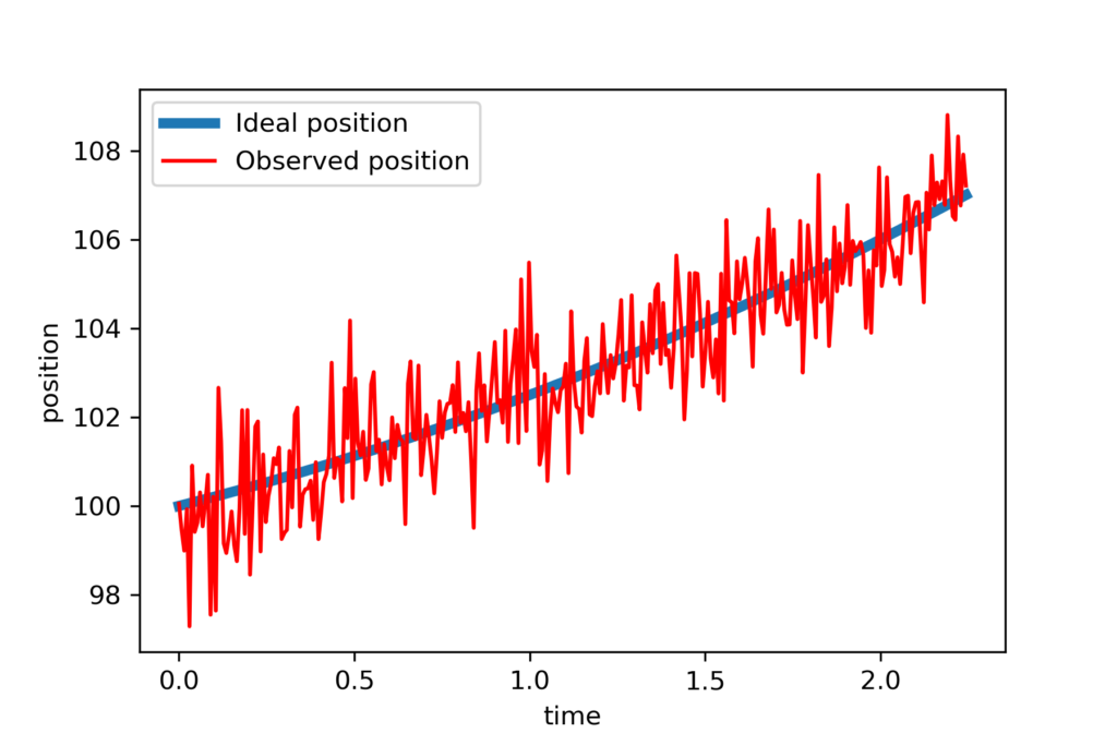
# verify the position vector by plotting the results
plotStep=300
plt.plot(simulationTime[0:plotStep],position[0:plotStep],linewidth=4, label='Ideal position')
plt.plot(simulationTime[0:plotStep],positionNoisy[0:plotStep],'r', label='Observed position')
plt.xlabel('time')
plt.ylabel('position')
plt.legend()
plt.savefig('data.png',dpi=300)
plt.show()

First, we import the necessary libraries as well as the class RecursiveLeastSquares. Then we assume “true” values of the initial position, initial velocity, and acceleration. These values are used in the code lines 20 and 21 to generate the data. Then on the code line 24, we corrupt the data with measurement noise. Finally, we plot the data. The figure below shows the data.

Next, we generate initial guesses of the parameters we want to estimate, and estimation error covariance matrix. Then we perform recursive estimation and plot the results.

x0=np.random.randn(3,1)
P0=100*np.eye(3,3)
R=0.5*np.eye(1,1)

# create a recursive least squares object
RLS=RecursiveLeastSquares(x0,P0,R)

# simulate online prediction
for j in np.arange(np.size(simulationTime)):
    C=np.array([[1,simulationTime[j],(simulationTime[j]**2)/2]])
    RLS.predict(positionNoisy[j],C)

# extract the estimates in order to plot the results
estimate1=[]
estimate2=[]
estimate3=[]    
for j in np.arange(np.size(simulationTime)):
    estimate1.append(RLS.estimates[j][0])
    estimate2.append(RLS.estimates[j][1])
    estimate3.append(RLS.estimates[j][2])
    
# create vectors corresponding to the true values in order to plot the results
estimate1true=initialPosition*np.ones(np.size(simulationTime))
estimate2true=initialVelocity*np.ones(np.size(simulationTime))
estimate3true=acceleration*np.ones(np.size(simulationTime))


# plot the results
steps=np.arange(np.size(simulationTime))
fig, ax = plt.subplots(3,1,figsize=(10,15))
ax[0].plot(steps,estimate1true,color='red',linestyle='-',linewidth=6,label='True value of position')
ax[0].plot(steps,estimate1,color='blue',linestyle='-',linewidth=3,label='True value of position')
ax[0].set_xlabel("Discrete-time steps k",fontsize=14)
ax[0].set_ylabel("Position",fontsize=14)
ax[0].tick_params(axis='both',labelsize=12)
#ax[0].set_yscale('log')
ax[0].set_ylim(98,102)  
ax[0].grid()
ax[0].legend(fontsize=14)

ax[1].plot(steps,estimate2true,color='red',linestyle='-',linewidth=6,label='True value of velocity')
ax[1].plot(steps,estimate2,color='blue',linestyle='-',linewidth=3,label='Estimate of velocity')
ax[1].set_xlabel("Discrete-time steps k",fontsize=14)
ax[1].set_ylabel("Velocity",fontsize=14)
ax[1].tick_params(axis='both',labelsize=12)
#ax[0].set_yscale('log')
#ax[1].set_ylim(0,2)  
ax[1].grid()
ax[1].legend(fontsize=14)

ax[2].plot(steps,estimate3true,color='red',linestyle='-',linewidth=6,label='True value of acceleration')
ax[2].plot(steps,estimate3,color='blue',linestyle='-',linewidth=3,label='Estimate of acceleration')
ax[2].set_xlabel("Discrete-time steps k",fontsize=14)
ax[2].set_ylabel("Acceleration",fontsize=14)
ax[2].tick_params(axis='both',labelsize=12)
#ax[0].set_yscale('log')
#ax[1].set_ylim(0,2)  
ax[2].grid()
ax[2].legend(fontsize=14)

fig.savefig('plots.png',dpi=300)

The code lines 1 and 2 are used to set the initial guess of and initial guess of the estimation error covariance matrix. Note that we are assuming a relatively large value of entries of the estimation error covariance matrix. This means that we do not have confidence in our initial guess of . Also, note that we also choose the value of the measurement noise covariance matrix. Our chosen value is different from the noise statistical properties (simulated noise standard deviation is 1 in our simulation). However, we assume a noise variance of 0.5. This actually a model uncertainty. We deliberately introduced this model uncertainty in order to make our estimation procedure realistic since, in practice, we often do not know a prior noise statistical properties. Then, in the code line 6, we create RecursiveLeastSquares object. The for loop in the code lines 9-11is used to make predictions by calling “predict()” method of the created object RecursiveLeastSquares. Finally, we plot the estimation results and show the convergence. Also, we compare the true value of our parameters with estimates. The results are shown in the figure below.

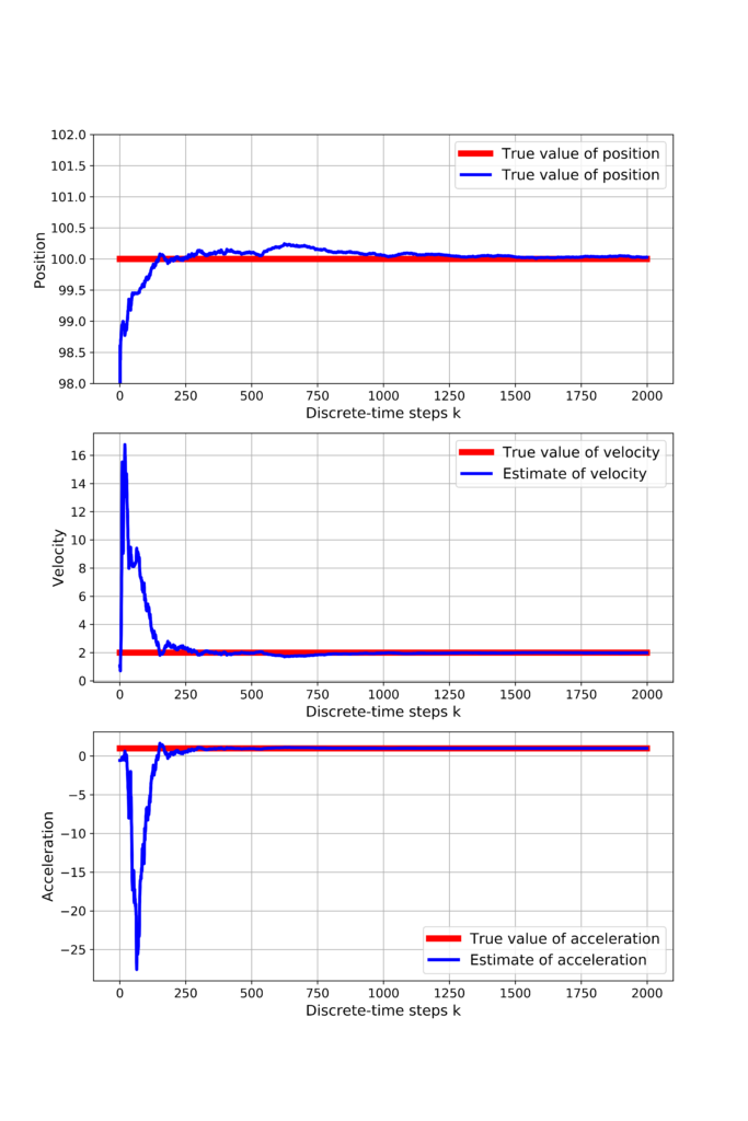
We can observe that all the estimates converge to the true values of parameters relatively quickly, despite the fact that the measurements are quite noisy. The GitHub page with all the codes is given here.