Clear and Concise Particle Filter Tutorial with Python Implementation- Part 1: Problem Formulation

In this estimation, control theory, machine learning, signal processing, and data science tutorial, we provide a clear and concise explanation of a particle filter algorithm. We focus on the problem of using the particle filter algorithm for state estimation of dynamical systems. Besides providing a detailed explanation of particle filters, we also explain how to implement the particle filter algorithm from scratch in Python. Due to the objective complexity of the particle filters, we split the tutorial into three parts:

1. Part 1. You are currently reading Part I. In this tutorial part, we define the particle filter estimation problem. We explain what is the main goal of particle filters and what particle filers are actually computing or better to say, estimating. We also clearly explain the concepts of state transition probability (state transition probability density function), measurement probability (measurement probability density function), posterior distribution (posterior probability density function), etc.
2. Part 2: In the second tutorial part whose link is given here, we present the particle filter algorithm.
3. Part 3: In the third tutorial part whose link is given here, we explain how to implement the particle filter in Python from scratch.

These tutorials are specially designed for students who are not experts in statistics and who are not experts in control theory. We thoroughly explain all the used statistics concepts. Nowadays, there is a trend not to thoroughly study theoretical concepts and quickly jump to Python scripts implementing algorithms, without first properly understanding the theoretical background of algorithms. If you follow such an approach, you will never be able to understand particle filters, and you will not even be able to understand the Python implementation of particle filters. To properly understand particle filters, you need to first properly understand important concepts from dynamical system theory, probability theory, and statistics. These concepts are thoroughly explained in this tutorial. Consequently, reserve some time and stay focused while reading this tutorial. Do not immediately jump to the second or third parts without properly understanding the material presented in this tutorial.

That is, THIS TUTORIAL IS NOT FOR STUDENTS WHO EASILY GIVE UP. PROPER UNDERSTANDING OF PARTICLE FILTERS REQUIRES EFFORT FROM THE STUDENT’S SIDE.

In this tutorial:

• We explain what are state-space models.
• We explain what are the process disturbance and measurement noise of state-space models.
• We explain what is a transition state probability of a state-space model.
• We explain what is a measurement probability of a state-space model.
• We explain what is a Markov process.
• We explain the classical state estimation problems, such as recursive and batch state estimation problems.
• We explain the main difference between particle filter estimation problems and classical estimation problems.
• We explain what is a posterior distribution in particle filter estimation problems.
• We explain what are particles in particle filter algorithms.
• We explain what are weights and state-space samples in particle filter algorithms.
• We provide an intuitive explanation of the approximation of posterior distribution by using discrete probability involving particles.
• We define the problem of estimating the posterior distribution by using particle filters.

The YouTube tutorial accompanying this tutorial is given below.

By the end of this tutorial, you will be able to understand these two important graphs that illustrate the particle filter problem formulation.

Also, by going through all 3 tutorial parts, you will be able to simulate a particle filter shown in the video below.

State Estimation By Using Particle Filters – Problem Formulation

First, we explain the concept of a state-space model of a dynamical system. Then, we introduce statistical distributions that are related to the state-space model. Finally, we define the state estimation problem for particle filters.

State-Space Models

First, we need to define what is a model of a dynamical system. In a fairly general form, models of dynamical systems are represented by the state and output equations:

(1)  

where is the state vector at the (discrete) time step , is the control input vector at the time step , is the process disturbance vector (process noise vector) at the time step , is the observed output vector at the time step , and is the measurement noise vector at the discrete time step . In the most general case, the functions and are nonlinear functions.

It is always important to keep in mind the following facts when dealing with state-space models of dynamical systems given by (1).

• The state of the system is usually not completely observable. We can only observe or sense the output of the system denoted by . The main purpose of state estimators is to estimate the state of the system by using the measurements of .
• The vector is the process disturbance vector. This vector is also called the process noise vector. The exact value of this vector is usually not known (unless we use a method to estimate its value). However, we can model the statistics of this vector. For example, we can model or estimate the mean and covariance matrix of the distribution describing the statistics of this vector. In practice, this vector can for example mathematically model stochastic state disturbances affecting the dynamics. Some researchers use this vector to take into account model uncertainties. We will talk more about the statistics of this vector in the next subsection of this tutorial.
• The vector is the measurement noise vector. In practice, the measurement process or sensors introduce noise in the observed variables. This vector is used to mathematically model the sensor or measurement process noise. Similar to the process disturbance vector, we do not know the exact value of the measurement noise vector. Instead, we can either model or estimate the statistical description of this vector. For example, we can model or estimate the mean and the covariance matrix of the statistical distribution of this vector. We will talk more about the statistics of this vector in the next subsection of this tutorial.
• The vector is the control input vector. We assume that the control input vector is perfectly known. This is because the control algorithm computes the numerical value of the control input vector. Here, there is an additional complication that we will simply ignore in this tutorial. Namely, the control input vector is computed by using the information from states and outputs at the past time steps. That is, this input is not independent of the statistics of the past states and outputs. This fact creates additional complications when deriving the estimation algorithms and when analyzing their behavior. For simplicity, in this tutorial, we completely ignore this fact.

For clarity and not to blur the main ideas of particle filters with too many details of complex nonlinear functions, in this tutorial and other parts of the tutorial series, we assume that the model (1) is linear and that it has the following form

(2)  

where , , and are state, input, and output system matrices. Everything explained in this tutorial can be generalized to a broad class of nonlinear systems.

Statistics and State Space Models

Here, we explain the statistics of random vectors in the state-space model (2). The proper understanding of the statistics of these vectors is important for the proper understanding and implementation of particle filters. Here, for clarity, we repeat the state-space model description:

(3)  

Here, for simplicity and presentation clarity, we assume that

1. The process disturbance vector is a Gaussian random vector. That is, the vector is distributed according to the Gaussian distribution which is also known as the normal distribution. We assume that the mean of is zero and that the covariance matrix is . In the general case, the mathematical notation for Gaussian random vectors is
   
   

   (4)  

   
   where this notation means that the vector is distributed according to the normal distribution with the mean of and the covariance matrix of . In the general case, a vector with the mean of and the covariance matrix of is said to be distributed according to . That is, the first entry in the notation is the mean of the vector, and the second entry is the covariance matrix.
2. The measurement noise vector is a Gaussian random vector. We assume that the mean of is zero and that the covariance matrix is . That is,
   
   

   (5)  

We introduced these assumptions to simplify the explanation of particle filters. However, particle filters can be used when random vectors have non-Gaussian probability distributions.

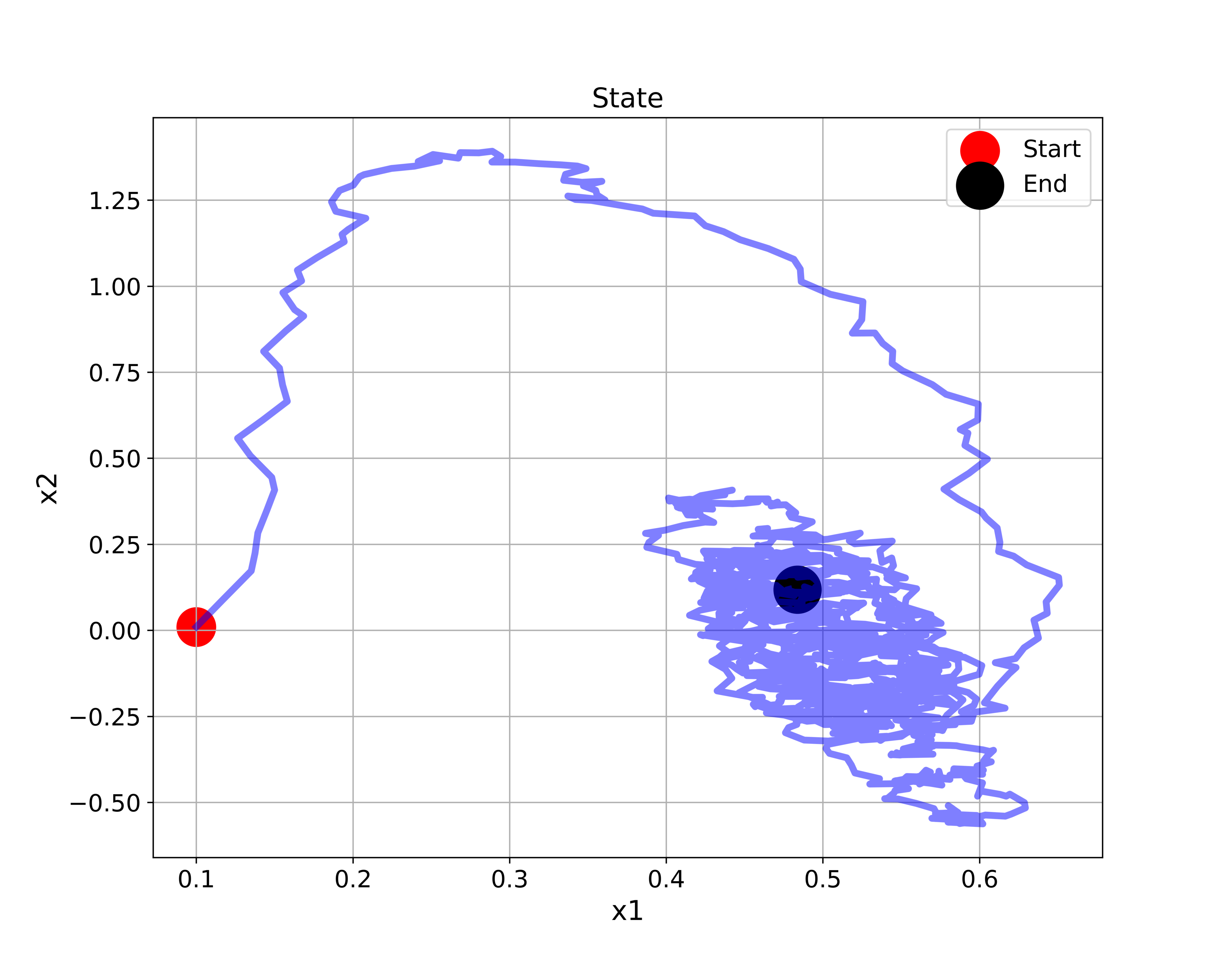
In our previous tutorial given here, we explained how to simulate the stochastic state-space model (3) in Python. It is a good idea to go over that tutorial in order to get yourself familiar with the simulation of random state space models. The simulated state-space trajectory is given below.

In Fig. 1 above, at every discrete-time step, we generate a random sample of the process disturbance vector from the normal distribution. If we would repeat the simulation from the same initial condition represented by the red circle, we would obtain a different state-space trajectory. This is the direct consequence of the stochastic nature of the state-space model.

Here is very important to properly understand the following. In (3), since the vector is random, for known values of and , the vector is also random! That is, the randomness of the process disturbance vector induces a probability distribution of . This probability is called the state transition probability. Other names for this probability are next-state probability or transition probability. The state transition distribution plays a very important role in particle filters. The probability density function of the state transition probability is denoted by

(6)  

This is a probability density function of a conditional probability. That is, this is a probability density function of a probability of under the assumption that the values of and are known and fixed.

Now, the main question is: What is the mathematical form of the state transition probability? Since the vector in the state equation of (3) is normally distributed, and since the state equation is linear, we conclude that the state transition probability belongs to the class of normal distributions. The mean of this distribution is computed from the state equation and is equal to

(7)  

The covariance matrix is equal to the covariance of . That is, the covariance of the state transition distribution is . From this, we conclude that the state transition distribution is a normal distribution with the mean of and with the covariance matrix of . The mathematical form of the state transition probability density function is

(8)  

where is the state dimension.

On the other hand, since the measurement vector is a random vector, the output measurement vector is a random vector. The probability of is called the measurement probability. The measurement distribution also plays a very important role in particle filters. The probability density function of the measurement probability is denoted by

(9)  

This is a probability density function of the conditional probability that is derived under the assumption that the value of is known and fixed. Now, the main question is: “What is the mathematical form of the measurement probability?” Since the output equation of (2) is linear and the vector is distributed according to the normal distribution, we conclude that the measurement probability belongs to the class of normal distributions. The mean of this distribution is and the covariance is .

Consequently, we conclude

(10)  

where is the dimension of the output vector.

Here, we need to explain an additional concept that you will need to understand in order to understand the derivation of the particle filter that we will present in the next tutorial. Namely, often in estimation and statistics literature, you will encounter the term “Markov process” or a “Markov chain”. Loosely speaking, a stochastic process is Markov if the state probability at the current time step depends only on the state (and known constants) from the previous time step. This means that the state sequence:

(11)  

is generated such that the probability of moving from the previous state to the current state only depends on the previous state . That is, the transition probability of a Markov process does not depend on the past states . From the mathematical point of view, this means that the probability density function of a Markov process must satisfy

(12)  

However, since an output equation participates in a state-space model description, for a state-space model to be a Markov state-space model, we also need an additional requirement. This requirement is that the output probability at the current time step depends only on the state (and known constants) at the current time step. This means that the output probability density function must satisfy

(13)  

Obviously, the linear state-space model (3) is a Markov state-space model.

State Estimation Using Particle Filters – Problem Formulation

Here again, for presentation clarity, we repeat the state-space model

(14)  

The standard notation for the state estimate at the time step is . That is, we use the so-called “hat” notation for state estimates.

To be able to understand the state estimation problem for particle filters, one first needs to understand the classical state estimation problem. The classical state estimation problem is to estimate the state at the current time step by using

1. State-space model of the system (14).
2. Past state estimates up to and NOT including the time step : , , , , .
3. Past observed outputs up to AND including the time step : , , , , .
4. Past control inputs up to and NOT including the time step : , , , , .

That is, the classical state estimation problem is to compute the state estimate by incorporating all available information up to the time step .

Generally speaking, the classical state estimation problem can be solved by using three approaches. The first approach is to use the batch mathematical formulation, where the state is directly estimated by solving an optimization problem involving a sequence of past input and output data. The most basic estimator that uses this idea is an open-loop least-squares observer which we explained in our previous tutorial:

• Easy Introduction to Observability and Open-loop Observers with MATLAB Implementation

The second approach is to recursively (sequentially or iteratively) estimate the state at the time step by using the past state estimate and past input information from the previous time step , as well as the output at the time step . The most popular recursive estimators are the Luenberger observer and Kalman filter. We covered these recursive estimators in our previous tutorials:

• Correct Explanation of State Observers for State Estimation of State-Space Models with Python Simulations
• Design and Test Observers of Dynamical Systems in MATLAB
• Kalman Filter Tutorial- Derivation of the Kalman Filter by Using the Recursive Least-Squares Method
• Disciplined Kalman Filter Implementation in Python by Using Object-Oriented Approach

The third approach is to combine the first and second approaches. The third approach is called moving horizon estimation. We will cover the moving horizon estimation approach in our future tutorials.

Most of the above-mentioned estimation approaches produce a single estimate of the state vector. That is, they aim at directly computing . Also, under the assumption that the process and measurement noise are Gaussian and under the assumption that the dynamics is linear, we can use these approaches to extract the covariance matrix of the estimation error and some other useful Gaussian statistics that can help us to evaluate and quantify the estimation uncertainty, and statistical properties of the estimate . However, when the measurement and process noise are not Gaussian and when the dynamics is not linear it becomes challenging to extract statistical information about the estimate and to quantify the estimation uncertainty.

On the other hand, particle filters use a completely different estimation paradigm.

Instead of mainly being focused on computing a single state estimate, particle filters aim at estimating a probability distribution or a probability density function of the state conditioned on the output observations and on past control inputs .

By using the Bayesian estimation terminology, this distribution is called the posterior distribution or posterior probability. The probability density function of the posterior probability is denoted by

(15)  

where and denote the sets of inputs and outputs

(16)  

In robotics literature, the posterior probability is also called the belief distribution. Also, some researchers call the posterior density as the filtering density. The vertical bar in the notation for the posterior probability density function (15) means that this posterior is computed by using the information available in the output and input time series.

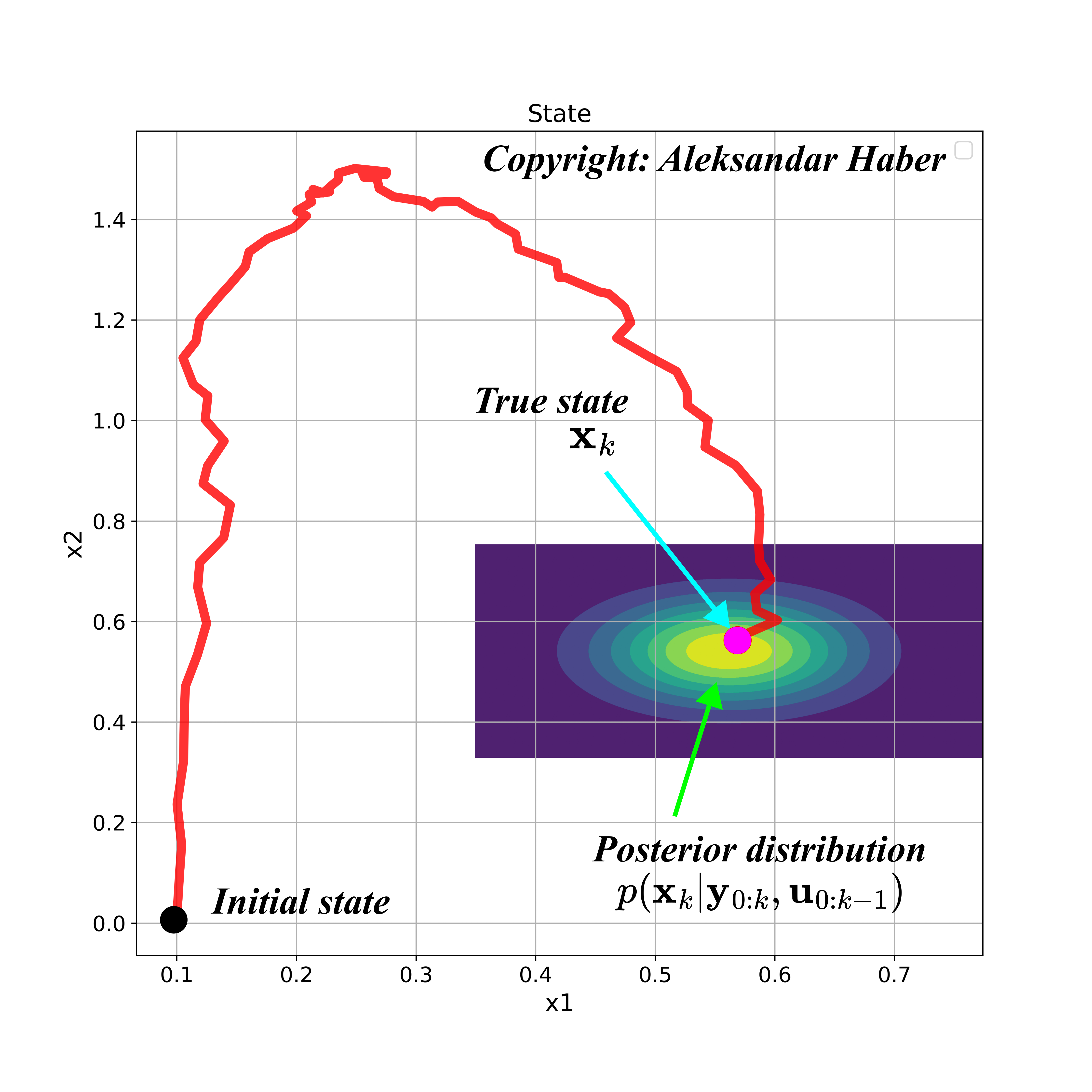
The figure below shows a simulated state-space trajectory of a second-order system, and a possible posterior distribution at the time step .

In Fig. 2 above, the posterior distribution is represented by the contour plot. The colors represent the values of the probability density function. The brighter the color is, the higher the value of the probability density function of the posterior distribution is.

The posterior probability encapsulates the complete statistical information about the posterior state. The knowledge of the posterior probability enables us to accurately compute important statistical quantities related to our estimate, such as the mean (which can serve as a form of estimate), covariance matrix, higher-order moments, mode, confidence intervals, etc. We can also formulate an estimate as some other statistical measure that is computed on the basis of the posterior probability density function. That is, the complete solution to the state estimation problem is the posterior probability or posterior probability density function.

Motivated by this, a particle filter estimation algorithm aims at reconstructing or estimating the posterior probability density function or posterior probability of state.

That is, in sharp contrast to the classical estimation algorithms that are mainly focused on computing a single state estimate (and possibly moments of distributions related to the estimation problem, however, this is often only feasible for normal distributions), the particle filters aim at reconstructing or estimating the complete posterior probability density of the state. This is very important to understand!

The output of the particle filter is a discrete approximation of the posterior probability density function. The output is a set of particles approximating the distribution. Let us now explain what are the particles in particle filters.

Generally speaking, a particle is defined by the state (also known as the state sample) and the associated weight (also known as the importance weight) that is usually denoted by . The particle is denoted by . The set of particles is denoted by

(17)  

The weights are normalized, such that . Loosely speaking, the weights tell us how important each particle or point (sample point) is. By knowing the weights , and state samples , we can approximate the posterior distribution as follows

(18)  

where is the symbol for the Dirac delta function. The Dirac delta function is shifted and centered at the sample .

In probability theory, the Dirac delta function is used to represent a distribution of discrete variables by using the probability density function of the continuous variables. That is, the Dirac delta function is used to extend the definition of the probability density function for discrete random variables. This is very important to understand. For example, let us assume that we have a discrete set of values (points) that some random variable can take: . Let the probabilities at these points be . The set of points, and probabilities, define a probability mass function , such that , . Then, the probability density function is defined by

(19)  

By using this probability theory fact, we can interpret the weights in (18) as the probabilities at the points of the discrete distribution approximating the posterior distribution. If you want to know more about the Dirac delta function and its use in probability theory and statistics, you can read this tutorial and this tutorial.

For example, let us consider a simple case. Let us assume that the samples are scalar (states are scalars), and let us assume that we only have particles: , , , and . For example, if weights are interpreted as probabilities of a discrete distribution, we have the probability of of the state being equal to , that is, .

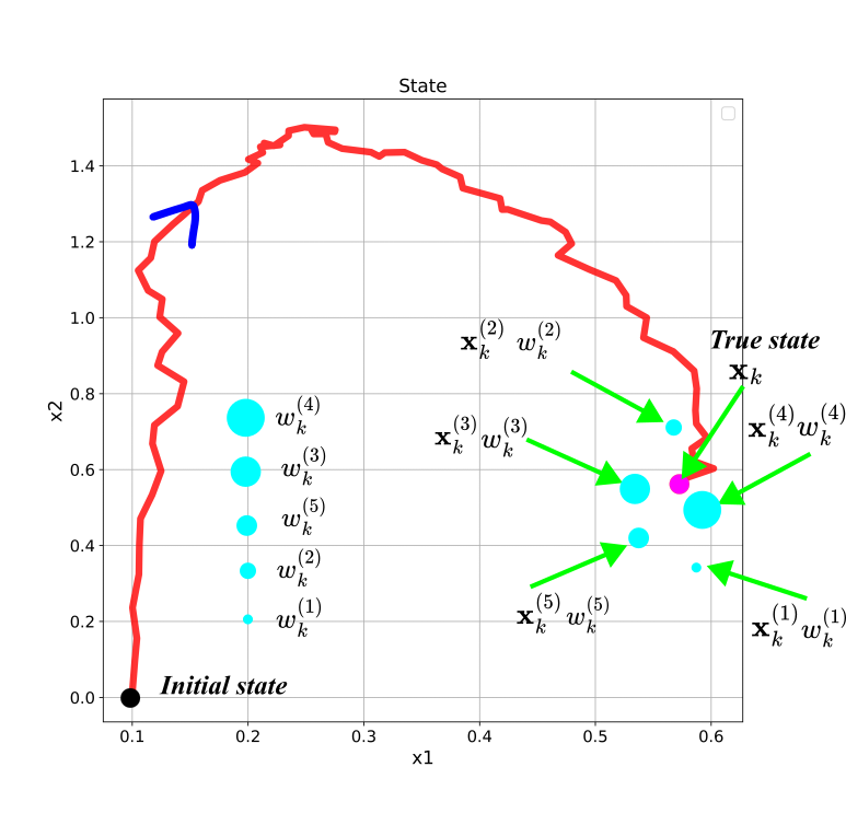
Next, let us consider another example, where the state is two-dimensional. The figure shown below shows the possible particles for the 2D state-space trajectory (see also the prior distribution shown in Fig. 2.). This trajectory is generated in Python by simulating the dynamics of a 2D dynamical system. The tutorial is given here.

In the figure above, the weight value is represented by the radius of the light blue circles. The larger the value of the weight is, the larger the radius of the circle is. The particle is closest to the true state, and consequently, it has the largest radius.

Generally, speaking the knowledge of the particles

(20)  

enable us to approximate any statistical moment (mean, covariance, and higher-order moments) or expectation of a nonlinear function of state by using this equation

(21)  

where is the expecation operator, and is in the general case, a nonlinear function. For example, if we want to compute the expectation, the function is simply equal to the state .

TO CONCLUDE: BY COMPUTING THE PARTICLES WE CAN APPROXIMATE THE POSTERIOR STATE DISTRIBUTION AND WE CAN APPROXIMATE ANY STATISTICS OF THE STATE!

Now we are ready to formulate the estimation problem for particle filters. We will formulate two problems.

ESTIMATION PROBLEM 1- GENERAL ESTIMATION PROBLEM FOR THE POSTERIOR DISTRIBUTION: By using the information about

1. State-space model of the system (14).
2. Transition probability .
3. Measurement probability .
4. Observed outputs and applied control inputs .
5. Initial guess of the particles
   
   

   (22)  

At every time step , estimate the set of particles (weights and state samples)

(23)  

that approximate the posterior distribution of the state

(24)  

The above estimation problem is defined in a batch estimation framework. The particle filter algorithm solves this problem recursively. Consequently, let us define the recursive estimation problem.

ESTIMATION PROBLEM 2- RECURSIVE ESTIMATION PROBLEM FOR THE POSTERIOR DISTRIBUTION: By using the information about

1. State-space model of the system (14).
2. Transition probability .
3. Measurement probability .
4. Observed outputs and the control input applied at the previous time step .
5. The set of particles computed at the time step
   
   

   (25)  

At the time step , compute the set of particles

(26)  

That recursively approximates the posterior distribution

(27)  

You should notice the main difference between these two problem formulations. The first problem formulation uses all the information up to the time instant to approximate the posterior distribution. The second problem uses the information from the previous time step and the current time step to approximate the posterior distribution.