In this control engineering and control theory tutorial, we provide a correct and detailed explanation of state observers that are used for state estimation of linear dynamical systems in the state-space form. We also explain how to implement and simulate observers in Python. The main motivation for creating this video tutorial comes from the fact that in a number of control engineering books and online tutorials, observers are presented from the mathematical perspective without providing enough practical insights and intuitive explanations of observers and state estimators. In contrast, in this control engineering tutorial, we provide an intuitive explanation of observers as well as a concise mathematical explanation. The observer developed in this tutorial belongs to the class of Luenberger observers. We use the pole placement method to design the observer gain matrix. We also explain the concept of duality between the observer design and feedback control problems. Finally, we design, implement, and simulate the observer in Python by using the Control Systems Library and the function place(). The complete Python code files developed in this tutorial are given here.
The YouTube tutorial accompanying this lecture is given below.

Motivational Example
As a motivational example, we consider a system shown in the figure below.

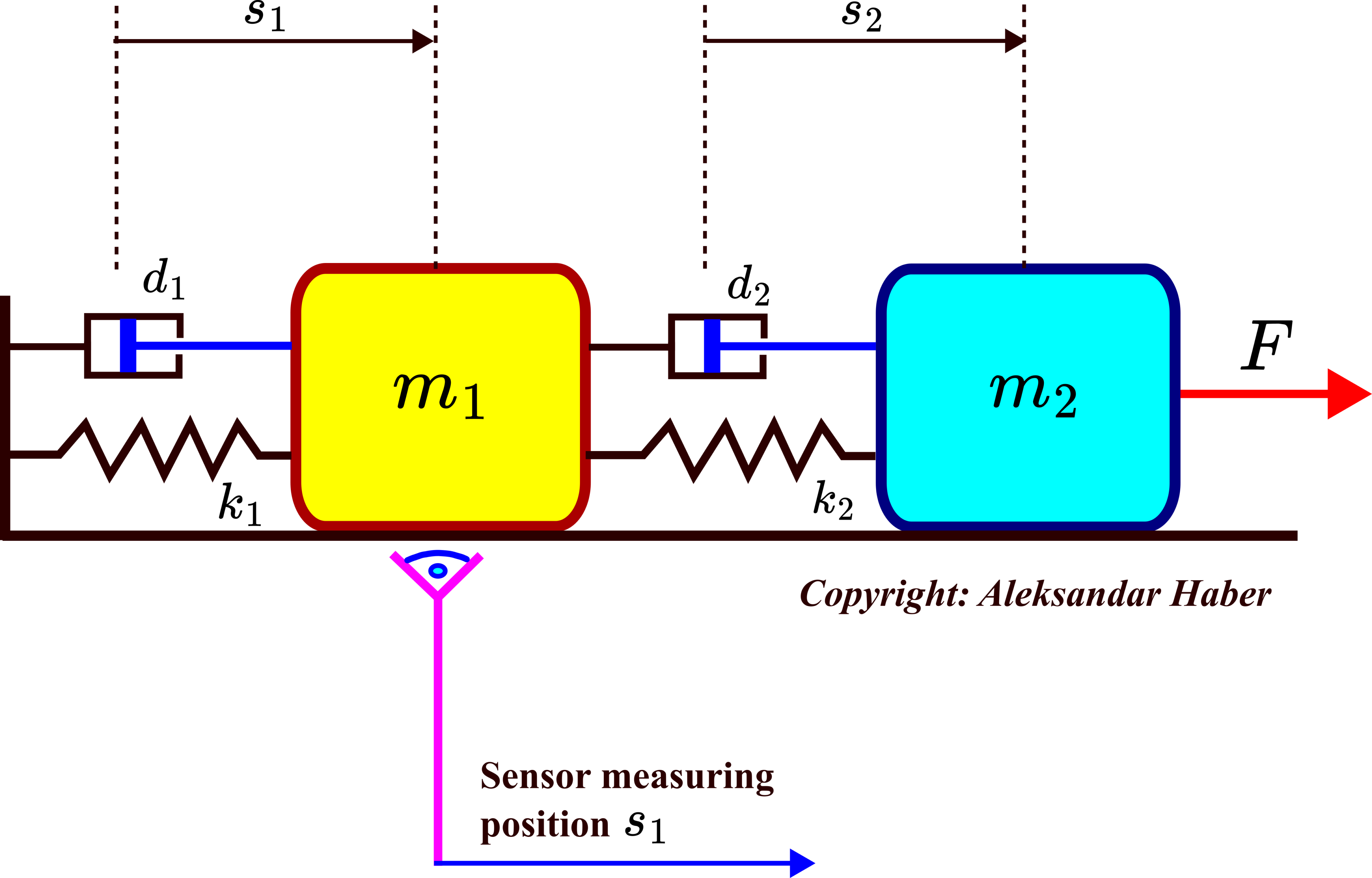
This system consists of two objects with masses 


(1) 

The complete state vector of the system is given by
(2) 

We want to provide the answer to the following question and solve the state estimation problem formulated below:
- Can we uniquely estimate the complete state vector by observing the time sequence of the position

- If yes, design a state estimator (observer) that will continuously reconstruct or estimate the complete state vector


To solve both of these two problems, we need to know the model of the system. In our previous tutorial given here, we derived a state-space model of the system and we explained how to simulate the state-space model in Python. The state space model has the following form
(3) 

where
(4) 

The answer to question 1 is related to the problem of observability of the state-space model (3). In our tutorial given here, we thoroughly explained the observability problem and the concept of observability of dynamical systems. Briefly speaking, if the system with its state-space model (3) is observable, then we can uniquely estimate the state vector 

Here, for presentation clarity, it is important to state the observability condition for linear systems in the most general form
(5) 
where 


(6) 

where it should be kept in mind that 
Let us now go back to the double mass-spring-damper system from the beginning of this tutorial. Since, 


(7) 

and we check the numerical rank of this matrix. The system is observable if and only if the rank of the observability matrix is equal to the state order. In our case, the state order is 

Now, we need to address the second problem, that is, we need to design an estimator that will continuously estimate the state vector from the sequence of the measurements of
Observers for State Estimation of Dynamical Systems
In this section, we address the second problem stated in the previous section:
Design a state estimator (observer) that will continuously estimate the complete state vector 
Here, for clarity, we repeat the state-space model
(8) 
With the state-space model (8), we associate a state observer that has the following form
(9) 

OVER HERE IT IS VERY IMPORTANT TO EMPHASIZE THAT THE OBSERVER (9) IS ACTUALLY AN ALGORITHM THAT CAN BE IMPLEMENTED IN CONTROL HARDWARE. OVER HERE, THIS ALGORITHM IS REPRESENTED AS A CONTINUOUS TIME-STATE EQUATION (DIFFERENTIAL EQUATION). IN PRACTICE, IT IS OFTEN DISCRETIZED AND IMPLEMENTED AS A DISCRETE-TIME FILTER IN CONTROL HARDWARE.
Here is the explanation of the observer vectors and matrices:


- The matrix


- The term

- The term


The observer diagram is shown below.

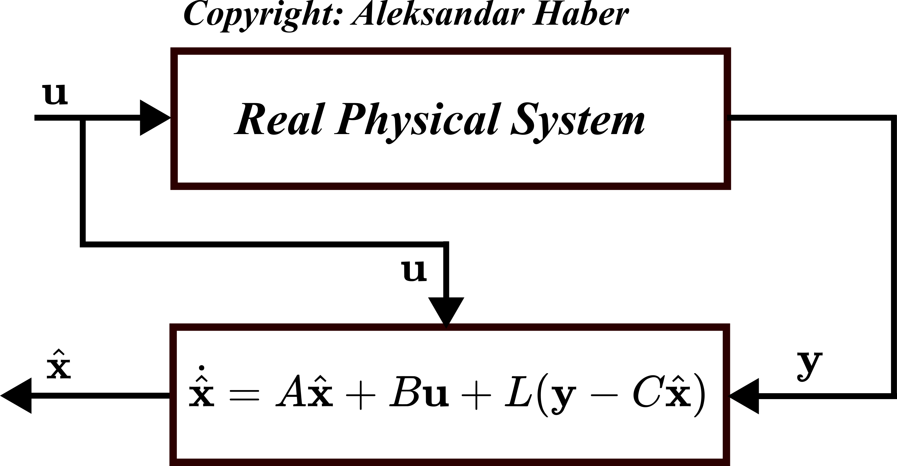
The observer inputs are the system control input 
Here, again, we will repeat the main goal of the observer.
The goal of the observer is to approximate and track the state of the system
So how to achieve this goal? We achieve this goal by properly designing the observer gain matrix 

Let us introduce the observer estimation error 

(10) 

The main goal of the observer is achieved by designing the matrix
(11) 

By substituting 


(12) 

The last equation is obtained by using (10) and by using the fact that 

(13) 

Now, the observer design problem is to design the matrix
The goal is to design the matrix 

Before we present a Python script for designing and simulating the observer algorithm. We need to address the following question.
Where to place the observer poles?
There are two schools of thought and two different opinions related to this important question.
- The observer poles must be two to five times faster than the feedback control poles in order to ensure that the observer estimation error (10) converges to zero much quicker than the control inputs. That is, we want our observer to quickly obtain a good estimate of the true system state, such that this state can be used in the state feedback control algorithm. Since in this case, the feedback control poles are slower than the observer poles, the closed-loop dynamics is primarily determined by the closed-loop control poles.
- The issue with the first approach is that in the presence of considerable noise and process disturbances, the fast dynamics of the observer closed loop poles can amplify the noise and disturbances. You can see that from the observer equation (9). The output of the system
Observer Design By Using Pole Placement and Observer Design and Simulation in Python
Over here, we explain how to design the observer gain matrix
Let 
(14) 

When defining the vector of desired pole locations, we need to keep in mind that if we specify a complex pole location, then we also need to have a conjugate pole that is symmetric with respect to the real axis.
To perform the pole placement, we use the Python Control Systems Library. In particular, we use the function place(). This function computes the matrix 

(15) 

has poles at prescribed locations. This function is used like this “place(A,B,p)”, where p is the list of desired poles (in our case the vector (14) ), and it returns the matrix
Now, how can we use this function to assign the poles of the closed-loop observer matrix
First of all, it is a very-well known fact that a square matrix and its transpose have the same set of eigenvalues. Consequently, the matrix
(16) 
and its transpose given by
(17) 

have identical eigenvalues. This means that we can assign the closed loop poles of (17) and these closed-loop poles will exactly be the closed loop poles of (16). It should be overved that the matrix 


Next, we need to explain how to simulate the computed observer. Let us look again at the observer equation
(18) 
We can write this equation like this
(19) 

This is a state equation, with
- the state matrix

- input matrix

- the input vector
(20)


By simulating the original system (3) for the known input
The system and observer simulations are given below. The first graph given below shows the step response of the system to the constant force equal to ![10 [N]](https://aleksandarhaber.com/wp-content/ql-cache/quicklatex.com-ce1ffd48c27039dff2dda6f269be1ef4_l3.png "Rendered by QuickLaTeX.com")


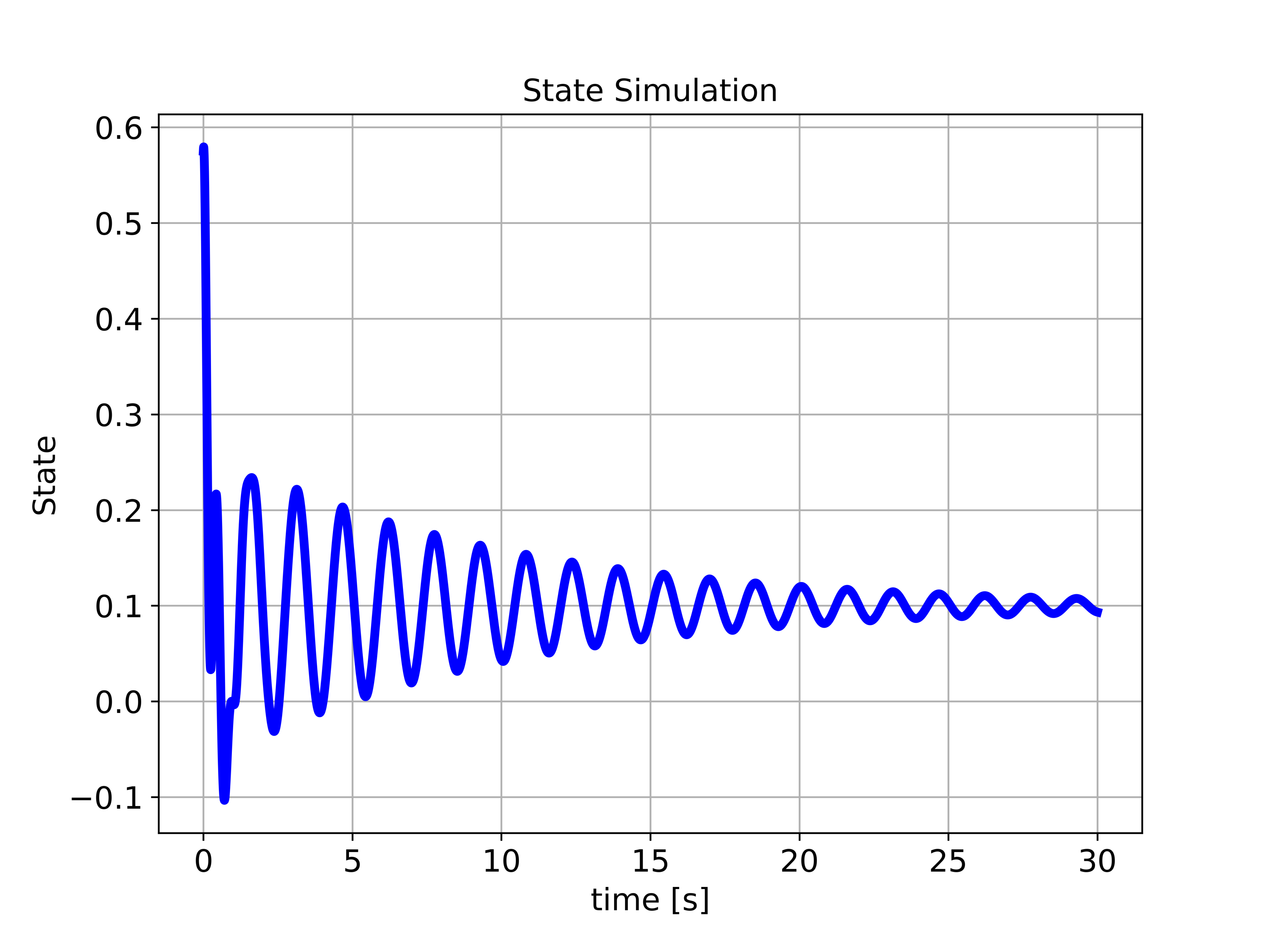
![10[N]](https://aleksandarhaber.com/wp-content/ql-cache/quicklatex.com-ad63ed9a6de7986dc1ff95983295af72_l3.png "Rendered by QuickLaTeX.com")
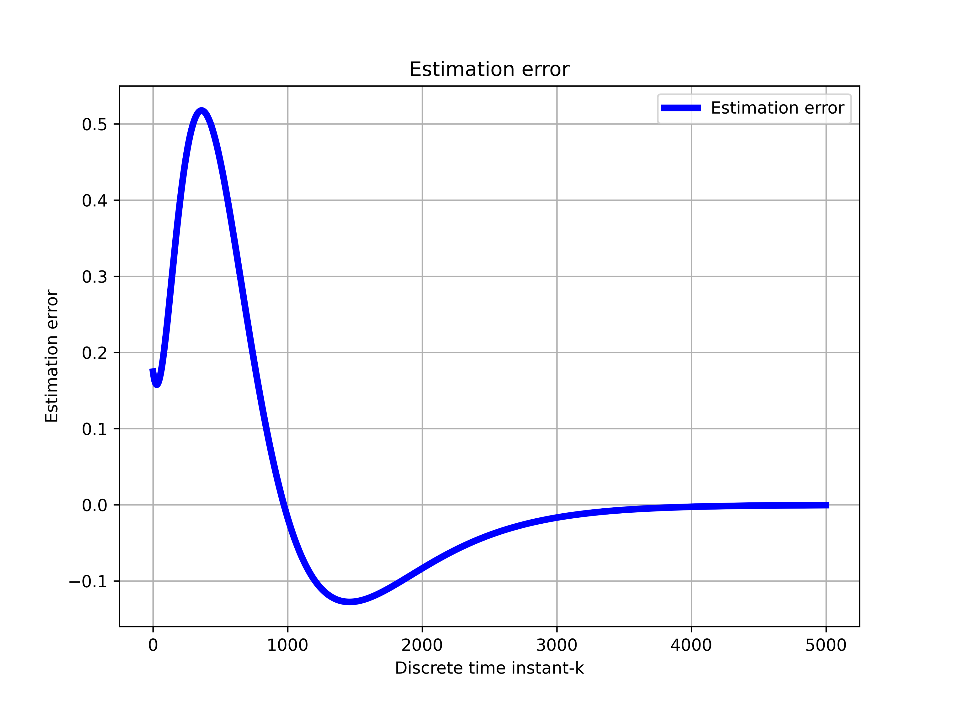
The figure below shows the convergence of the observer. We assumed an arbitrary initial condition of the observer. That is, we assumed an arbitrary initial guess of the state. The time behavior of the observer state variable 

We can observe that the state estimate