Correct and Intuitive Explanation of Observability of Linear Dynamical Systems

In this control engineering and control theory tutorial, we address the following problems and questions related to observability of linear dynamical systems

1. What is observability of linear dynamical systems?
2. How to properly and intuitively understand the concept of observability of dynamical systems?
3. How to test the observability of dynamical systems?
4. What is the connection between observability and conditions for the unique solution of systems of linear equations?

This tutorial is split into two parts. In the first part, we derive and thoroughly explain the theoretical conditions, and in the second part, we explain how to test observability of a system in Python.

Here is the motivation for creating the observability tutorial. The observability of dynamical systems is one of the most fundamental concepts in control engineering that is often not properly explained in control engineering classes. For example, it often happens that students/engineers immediately start designing observers/Kalman filters/particle filters without even testing observability. When the filter is not working, they start to scratch their heads and waste a significant amount of time checking the written code and trying to find a bug. In fact, you cannot uniquely estimate the system state if the system is not observable. This means that you cannot design an estimator for an unobservable system. Or you can, but only for the observable part of the system state (there is something called a triangular decomposition that reveals the observable subspace).

Then, another pitfall is that people often blindly memorize the observability rank condition without understanding the physical meaning of this condition and without truly understanding the observability concept. In fact, observability is nothing less than a fancy name invented by control engineers in the ’60s for the existence and uniqueness of the solution of a linear system of equations that appear when we “lift” the system dynamics over time. In fact, most of linear control theory is nothing less than applied linear algebra.

Observability analysis is also important for sensor placement problems, in which we are trying to maximize our estimation performance by placing the sensors at the proper locations in the system. In the tutorial presented below, we thoroughly and clearly explain the concept of observability and how to test observability by testing the existence and uniqueness of the solution of a linear system of equations.

The YouTube tutorials accompanying this webpage tutorial are given below.

Before we start with explanations, let us motivate the problem with the following example shown in the figure below.

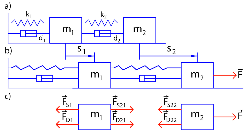
This is a system composed of two masses connected by springs and dampers. This is a lumped model of a number of physical systems that exhibit oscillatory behavior. The state variables are

• – position of the first mass.
• – velocity of the first mass.
• – position of the second mass.
• – velocity of the second mass.

The state vector is

(1)  

For more details about state-space modeling of the double mass spring damper system, see this tutorial.

Sensors are usually expensive and in addition, they complicate the mechatronics design of the system. We would like to minimize the number of sensors, while at the same time, achieving the control objective. On the other hand, ideally, we would like to observe all the state variables such that we can use them in a state feedback controller. The observability analysis of this system can provide us with the answers to the following and similar questions:

• Can we reconstruct the complete state vector by only observing the position state variable ? That is, can we compute the velocity of the first mass, as well as the position and velocity of the second mass by only observing the position of the first mass?
• If not, then, how many entries of the state vector do we need to directly observe in order to reconstruct the complete state vector?
• How many data samples of the observed variable do we need to have to completely reconstruct the state?

The easiest approach for understanding observability is to start from a discrete-time state-space model given by the following equation

(2)  

where and are state and output system matrices, is state, is the output, and is a discrete-time instant.

In a practical scenario, the vector is a vector of quantities that are observed by sensors, and the state is either a physical state (for example involving mechanical quantities) or the state is linearly related to the physical state through some matrix which is usually known as a similarity transformation.

The first question is: Why is it easier to understand the observability concept by considering discrete-time systems?

This is because it is easier to propagate the dynamics and equations of discrete-time systems over time. Namely, we can establish recursive relationships connecting different quantities at different time steps. We just perform back-substitution to relate quantities at different time intervals. This will become completely clear by the end of this tutorial. Here, we will briefly illustrate this. For example, by starting from the time instant and by recursively substituting states by using the state-space model (2), we obtain

(3)  

where is a positive integer. For linear continuous-time systems, it is more challenging to establish such relationships since we need to use integrals and differential calculus. For example, a continuous-time equivalent to the last equation in (3) is

(4)  

where is a continuous-time system matrix of the linear system , and is the initial state. The derivation of the equation (4) involves a relatively complex linear algebra and differential vector calculus.

The second question is: Is there a reason why we are not taking into account inputs when analyzing observability?

The answer is that known control inputs can easily be included as known quantities when analyzing observability, and we can subtract their effect from the observed outputs, and the resulting quantity can be used to derive the observability condition which is practically independent of the inputs. That is, the inputs do not affect the observability condition, and when analyzing the system observability, the inputs can be completely neglected.

Let us continue with the explanation of observability. Here is a formal definition of observability that can be found in many control theory books:

Definition of Observability: The state-space model

(5)  

is observable if any initial state of the system, denoted by can be uniquely determined from the set of output observations , where is a positive integer.

From this definition, we can conclude that the observability problem is closely related to the problem of estimating the state of the system from a sequence of output measurements. Secondly, we can observe that in the definition of observability, there is a parameter . This parameter is the length of the observation horizon. Its length generally depends on the number of observed outputs of the system, the structure of the system matrices and , and on the state dimension. There is a common misconception among control engineers that needs to be at least equal to ( is state dimension of the system) to make the system observable. To show this, let us consider the following example

Example 1: Is the following system observable

(6)  

where and are non-zero constants. Here, we directly observe scaled state variables since the matrix is a square by matrix. In addition, due to the fact that the constants and are non-zero, the matrix is invertible. From (6), we have

(7)  

This is a system of two equations with two unknowns (the entries of the initial state vector ). Since the matrix is invertible, there is a unique solution given by the following equation

(8)  

This example shows that we can actually uniquely estimate the initial state of the system by using only a single initial measurement of the system output. This is the direct consequence of the fact we are directly observing all (linearly scaled) state variables.

Let us now form the so-called lifted state-space description. The description is called “lifted” since we lift the state-space model over time to obtain a batch vector consisting of output samples. From (2) we have

(9)  

These equations are obtained by back substitution of the state equation of (2). Namely, from the state equation, we have

(10)  

The equation (9) can be written in the vector form

(11)  

Or more compactly

(12)  

where

(13)  

Here we need to explain the following

• The matrix is the step observability matrix.
• The vector is the step lifted output vector.

The equation (12) represents a system of equations with the unknowns that are the entries of the vector . From the derivations presented above, we can observe that the observability problem is equivalent to the problem of the existence and uniqueness of the system of equations (12).

We need to determine the conditions that will guarantee that this system of equations will have a unique solution.

In order to find the correct value for , let us analyze the dimensions of the system (12). This system has to have at least as many equations as the number of unknowns. We have in total equations and unknowns. We can also allow for more equations than unknowns. This means that the necessary condition is that . In the case of Single-Input-Single-Output (SISO) systems, we have that , and consequently, we have that . In the case of Multiple-Input-Multiple-Output (MIMO) systems, depending on , we can allow , as long as the underlying linear system of equations has at least the number of equations equal to the number of unknowns. However, since we want to derive the general condition that will be applicable to both SISO and MIMO systems, we will take . But, do we really need to select such that ? The answer is NO. There is a theorem called Cayley-Hamilton Theorem telling us that every matrix satisfies its characteristic polynomial. This means that we can express the powers of , where as linear combinations of powers of smaller than . This implies that any block row of the observability matrix after the block row can be expressed as a linear combination of previous rows.

Taking this analysis into account, we select . Then, our system has the following form

(14)  

where

(15)  

Now, we have to address the following question:

What is the condition that the matrix needs to satisfy such that this system has a unique solution?

The following theorem answers our question.

Observability Condition Theorem: The system of equations (14) has a unique solution if and only if

(16)  

That is, the system is observable if and only if the condition (16) is satisfied.

In words, if the matrix is a full-column rank matrix, then the system is observable. And the other way around, if the system is observable, then the matrix is a full column rank matrix. Here, we will only prove that the rank condition (16) will guarantee the observability of the system.

Let us assume that the condition (16) is satisfied. Then, by multiplying the equation (14) from left by we have

(17)  

Since the condition (16) is satisfied, the matrix is invertible, and consequently, the system of equations (17) has a unique solution, and the solution is given by the following equation

(18)  

Here, one more important thing should be mentioned. Consider this least-squares minimization problem

(19)  

Under the condition that the matrix has a full column rank, the solution is given by the following equation:

(20)  

That is precisely the equation (18). From this, we can observe that there close relationship between observability, least-squares solution, and state estimation.