Simple Discrete-time Model of Mobile Robot for Localization, SLAM, and Dead Reckoning

In this robotics and control engineering tutorial, we explain how to develop a simple discrete-time model of a mobile robot that can be used for the development of algorithms for localization, Simultaneous Localization And Mapping (SLAM), and dead reckoning.

We develop a discrete-time kinematics model and we explain several important aspects of this model. This model is used in our other tutorials for the development of robotics algorithms. This is arguably the simplest possible model of a mobile robot. For simplicity and clarity of this tutorial, we focus on a differential drive mobile robot introduced in our previous tutorial given here. Consequently, we strongly suggest to the reader of this tutorial to first thoroughly read and understand the material presented in our previous tutorial.

Although simple, the model developed in this tutorial can still be used in practical applications and the modeling ideas presented in this tutorial can be used as an inspiration to develop models of robots with various configurations.

We use two approaches to develop the discrete-time kinematics model. Both approaches result in the same discrete-time model. The first approach is based on the direct discretization of the continuous-time model of the robot kinematics. The second approach uses simple trigonometry and physical intuition to develop the model. The YouTube tutorial accompanying this tutorial is given below.

Continuous-Time Model of Mobile Robot

The figure below shows a graphical representation of a differential drive robot introduced in our previous tutorial given here.

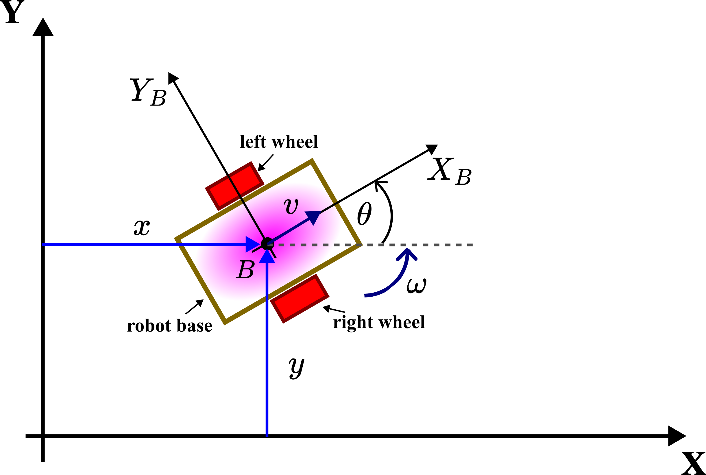
The robot consists of the robot base with two active (actuated) wheels and a third passive caster wheel. The third passive caster wheel provides the stability of the robotic platform (passive means that is not actively actuated, however, the wheel can still move around two perpendicular axes). This third wheel is not shown on the graph for clarity. We introduce the following quantities:

• Inertial coordinate system – (denoted by uppercase letters and ). This coordinate system is fixed.
• Body coordinate system – (denoted by uppercase letters and ). The body coordinate system is also called the body frame. This coordinate system is rigidly fixed to the robot body or robot base. Its center is at the point . Usually the point is the center of the mass or the center of the symmetry of the robot body or the robot base. The body coordinate system moves together with the robot.
• The coordinates and are horizontal and vertical positions of the body coordinate system – with respect to the inertial coordinate system –.
• The angle is the angle that the body coordinate system makes with the axis of the inertial coordinate system. That is, the angle is the rotation of the body coordinate system with respect to the inertial coordinate system. The angle is called the orientation angle or angular orientation. This angle is also called the bearing angle (or simply bearing) or heading angle (or simply heading). Since the body coordinate system is firmly attached to the robot body the angle is the rotation of the robot body.
• is the instantaneous velocity of the center of the body frame.
• is the instantaneous angular velocity of the robot.

Next, we need to define what is a robot pose. The (robot) pose is the vector defined by

(1)  

The (robot) pose completely defines the position (location) and orientation of the robot with respect to the fixed inertial frame –. From a purely geometrical point of view, the pose defines the location and orientation of the body frame – with respect to the inertial frame –. The pose is also called the kinematic state. The reason for this will be explained later on.

The precise knowledge of the robot pose is important for a number of reasons. First of all, it determines the precise location and orientation of the robot in space. Secondly, the robot pose is used for feedback control. Finally, robot pose information is used in other robotic algorithms, such as path planning, obstacle avoidance, and SLAM algorithms.

In our previous tutorial given here, we derived the continuous-time kinematics model describing the robot motion

(2)  

This model relates the instantaneous velocity and the current orientation angle of the robot with the change of the robot pose in the inertial coordinate system. Here, it is very important to understand that this model is developed by using only kinematics reasoning without taking into account the robot dynamics (mass and forces). In the sequel, we develop the robot model by discretizing this kinematics model by using the forward Euler method. Of course, the forward Euler method is only one among a number of discretization approaches. The main reason for using the forward Euler method is its simplicity and ease of implementation. On the other hand, to achieve a relatively good accuracy of the model obtained by using the forward Euler method, we need to select a small discretization step. Also, the forward Euler method might suffer from the stability issues. Some alternative approaches that achieve better modeling accuracy are the trapezoidal discretization method, backward Euler method (which has better accuracy and stability properties than the forward Euler method), trapezoidal implicit method, and the Runge-Kutta method. However, such methods result in mathematically complex models that might significantly increase the computational burden of robotics algorithms.

Derivation of the Robot Model by Using Discretization

Here, we obtain the robot model by using the forward Euler discretization. By using the forward Euler method, we discretize the time derivatives of , , and in the model (2), as follows

(3)  

where is the discretization step, is the discrete-time instant, and and are the horizontal and vertical coordinates of the center of the robot body frame at the discrete-time instant , that is, and . Similarly, is the orientation of the robot body frame at the discrete-time instant , that is, . Next, by using the forward Euler method and by substituting equations (3) in (2), and by replacing the approximation symbols with equality symbols, we obtain

(4)  

where is the instantaneous velocity at the discrete-time instant , and is the instantaneous angular velocity at the discrete-time instant . Here, it is implicitly assumed that the instantaneous velocity and angular velocity are constant between the discrete-time instants and .

From (4), we obtain the discretized kinematics model of the robot

(5)  

Next, we need to observe the following

• The product is the distance traveled in the direction of the velocity vector (the velocity vector is actually determined by the intensity given by and direction determined by the angle ). It should be kept in mind that the velocity vector is constant between the time instant and . The distance traveled between the time instant and is denoted by
  
  

  (6)  

• Since is the angular velocity, the product is the rotation angle of the robot body between the discrete-time instant and . We denote this angle by
  
  

  (7)  

Finally, by using (6) and (7), the final discretized model of the robot kinematics takes the following form

(8)  

Derivation of the Robot Model by Using Trigonometry and Physical Intuition

First, let us analyze the discrete-time model (8) obtained by using the forward Euler method. If we ignore the last equation in (8), the resulting two equations

(9)  

describe the translation of the robot body along the direction of the instantaneous velocity vector, where the orientation angle remains constant. On the other hand, if we ignore the first two equations in (8), and if we only consider the last equation

(10)  

then, this equation describes the rotation for the angle of . That is, the motion is decomposed (decoupled) into translation and rotation. This is a very well-known fact in kinematics and dynamics of motion of rigid bodies in a plane. Namely, the complex motion of a body in a plane from one pose to another can be decomposed into translation and rotation.

Let us not use this principle to rederive the kinematics model (8) by using a more intuitive approach that does not explicitly rely upon the model discretization.

We formally decompose the motion of the robot from the starting point (at the discrete-time ) to the endpoint (at the discrete-time instant ) as follows

• From the starting point (location at the discrete-time instant ) to the endpoint (location at the discrete-time instant ), the robot moves along a straight line. That is, during the motion from the point to the point , the orientation angle is constant, and the position coordinates and are changing.
• At the point , the orientation angle is changed, such that the orientation becomes .

This is just a formal mathematical decomposition of the motion, since in practice, the actual motion between the two points might not look like this. This is an approximation of the motion that enables us to mathematically analyze the geometry and kinematics of motion. However, if the time interval between the time instants and is relatively small this formal decomposition relatively accurately approximates the true motion. Also, it is important to keep in mind that at the time instants and the locations and orientations correspond to the real locations and orientations of the robot. What happens in between the time instants and cannot be exactly modeled unless a more complex mathematical model is used.

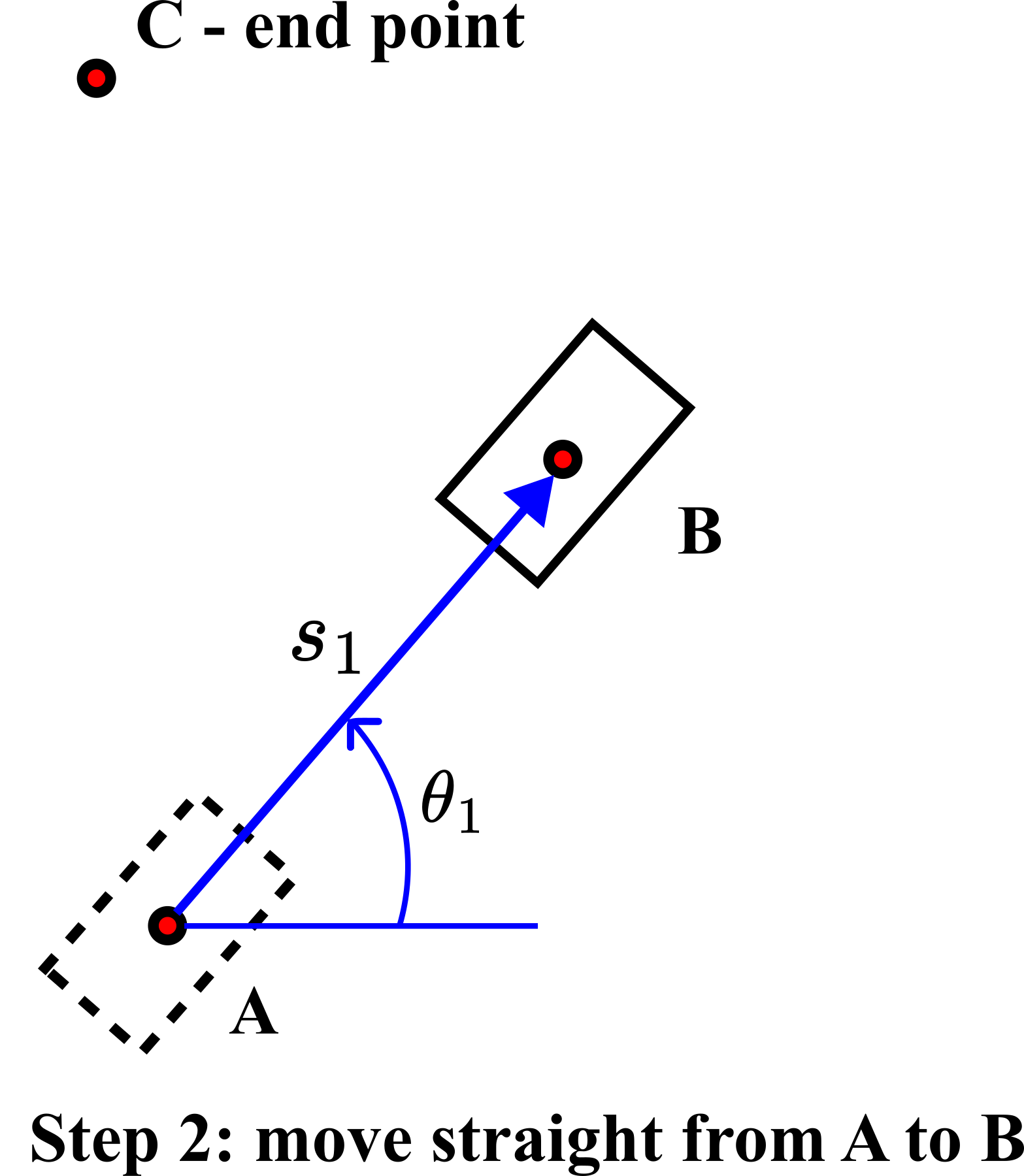
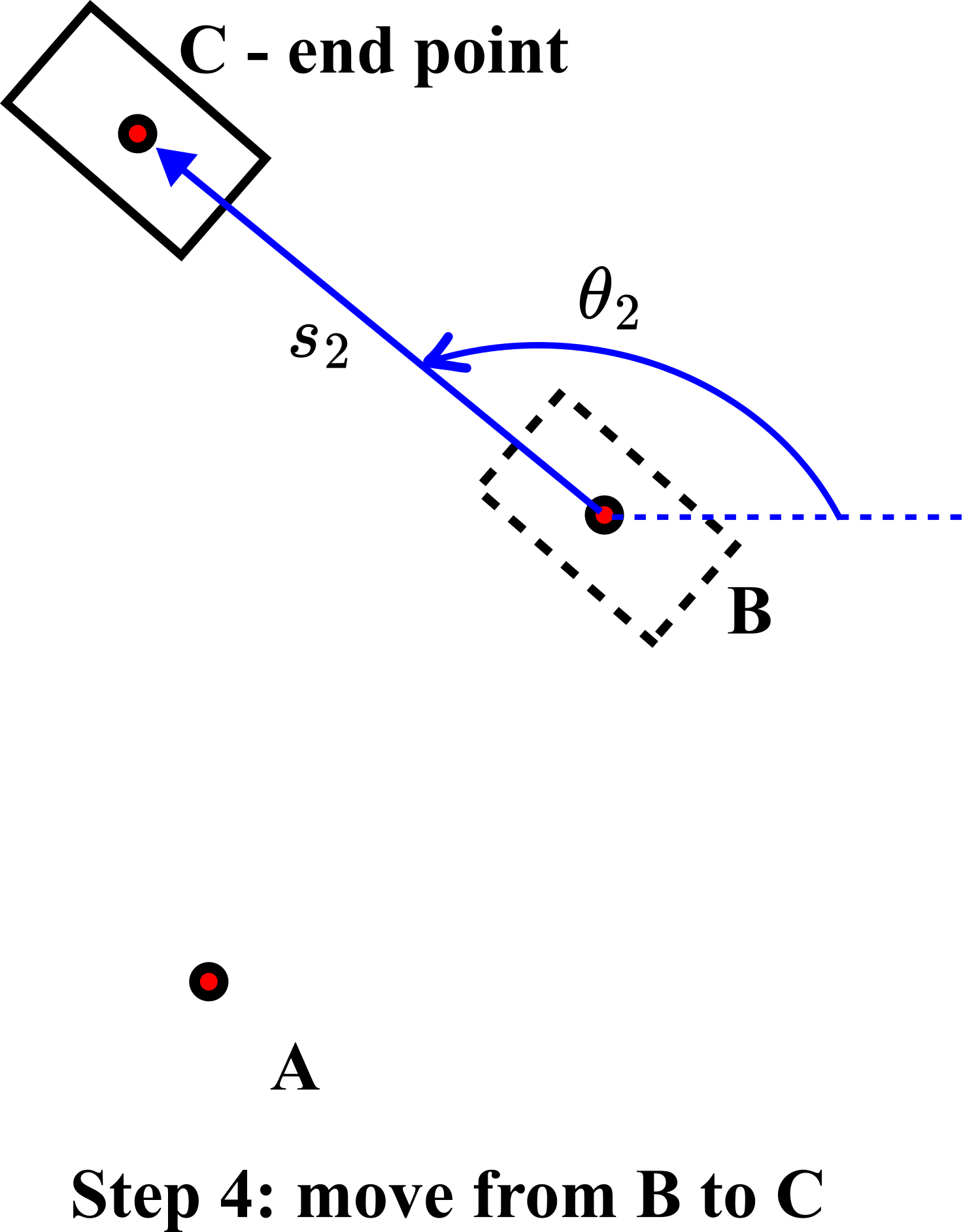
To repeat, from the mathematical point of view, the motion is decomposed into a series of straight-line motions and orientation changes. Let us illustrate this with the example shown in the figure below.

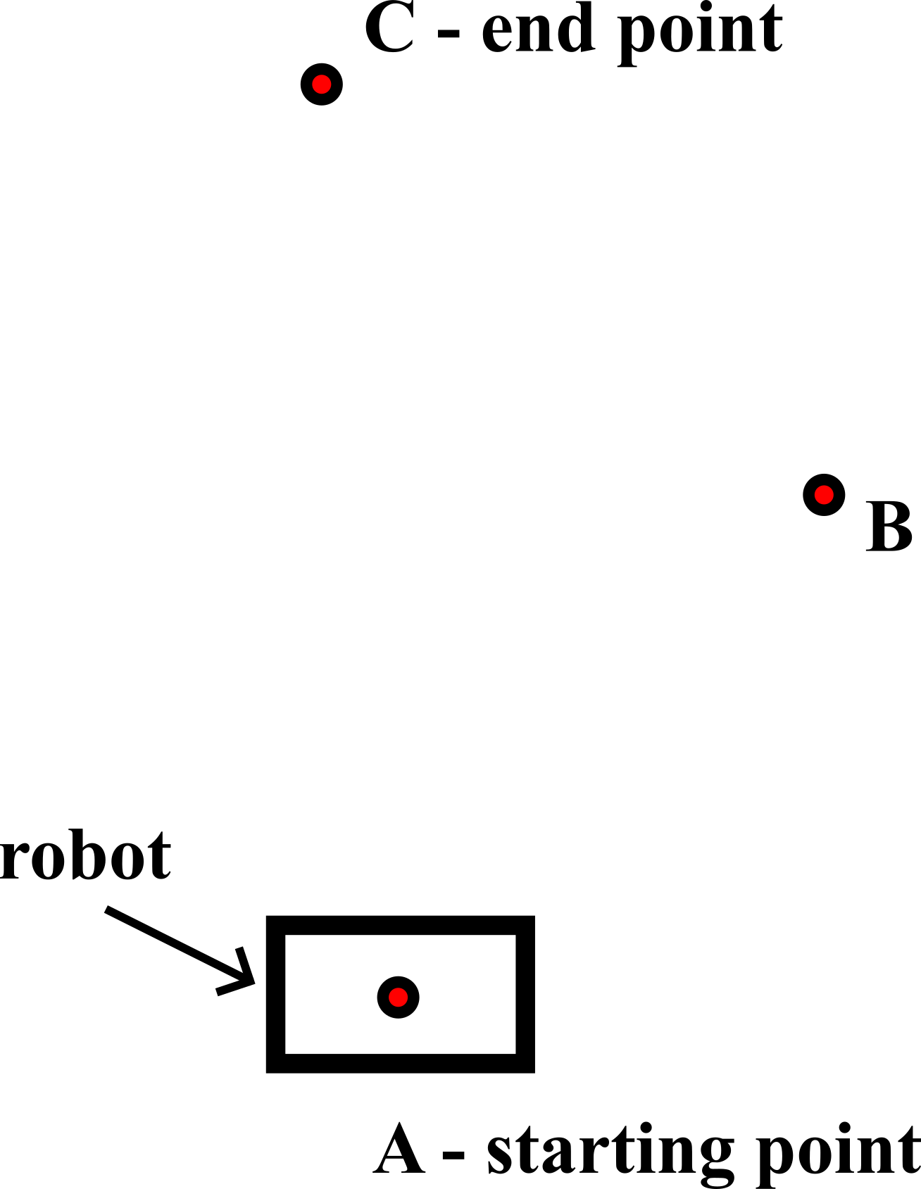
The goal is to move from the point to the point by visiting the intermediate point . The first step, while we are still in the point , is to adjust the orientation , such that the robot can move along the straight line from the point to the point . This is shown in the figure below.

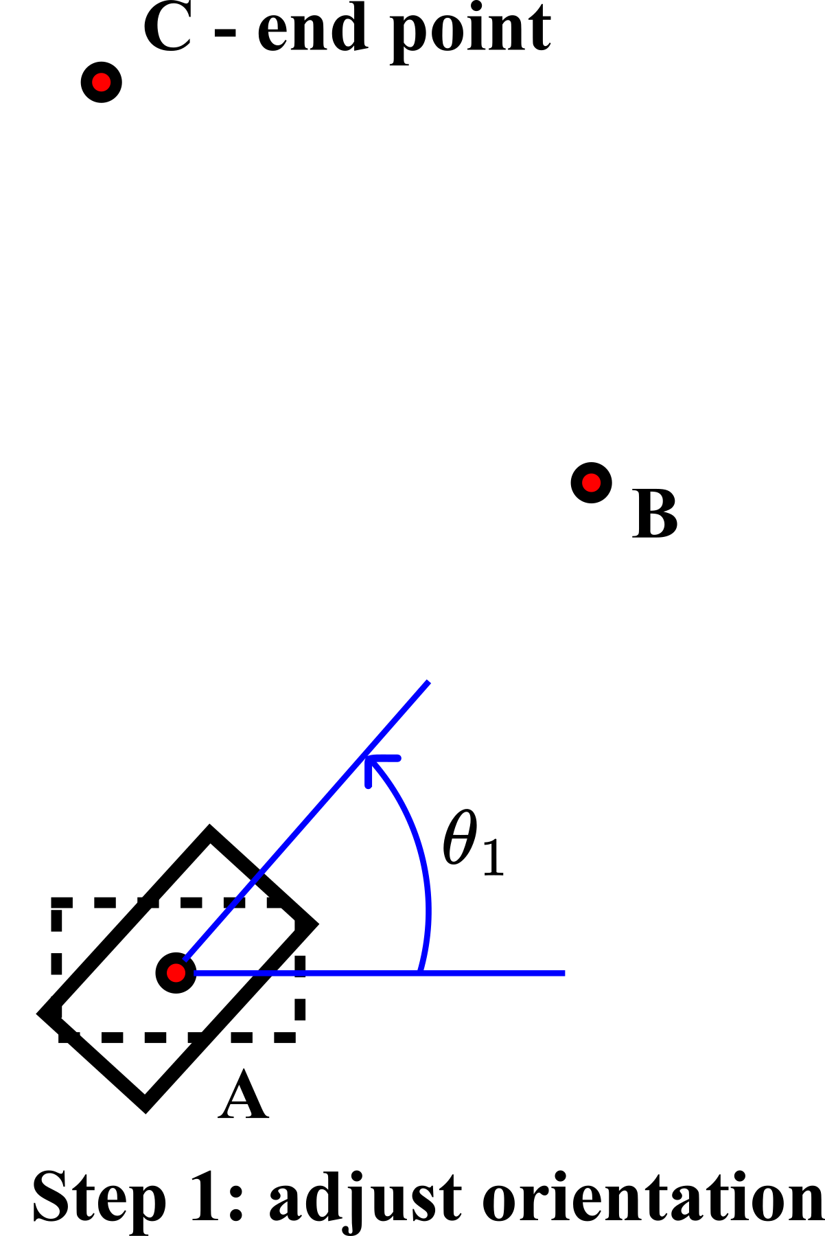
In step 2, we move from the point A to the point along the straight line for the distance . This is shown in the figure below.

In step 3, we adjust the orientation of the robot for the angle such that we can move along the straight line from the point to the point .

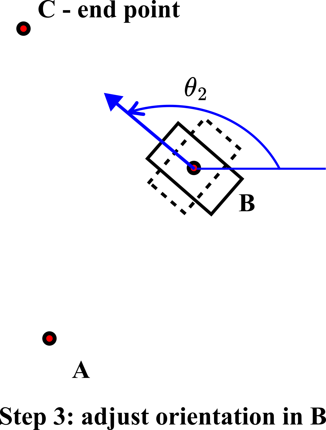
In step 4, we move along the straight line from the point to the point for the distance .

Next, we develop the kinematics model of the robot that mathematically describes this motion. Consider the figure shown below.

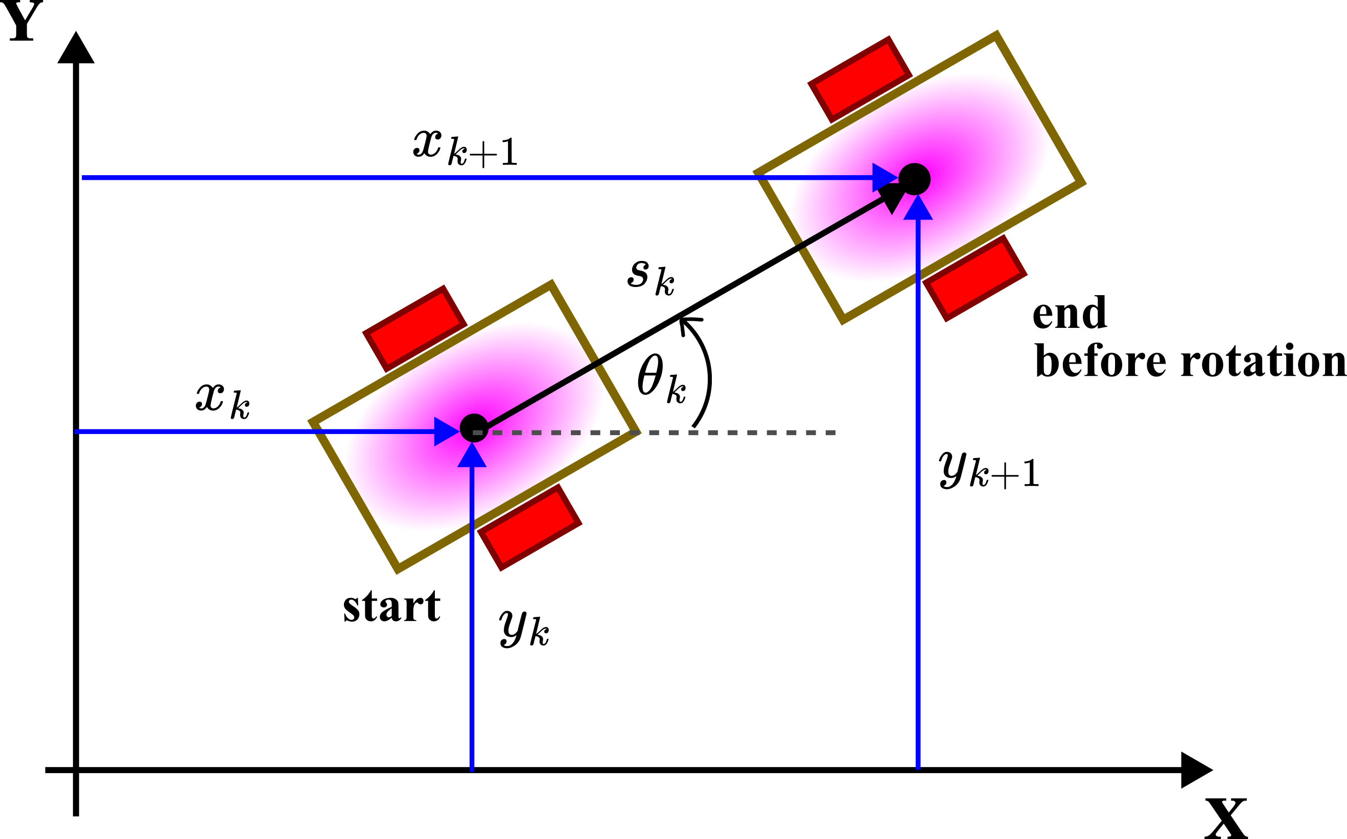
Here, we remind the reader that and denote the and coordinates of the center of the robot body at the discrete time instant . That is,

(11)  

where is the discretization step. That is, we look at the location of the robot at the discrete-time instants . Similarly, we have previously defined as follows

(12)  

From the discrete-time instant to the discrete-time instant , the robot travels from the start to the end position shown in the figure above. During that time interval, the robot had traveled the distance of . This is precisely the distance introduced in (6). Under the assumption that the orientation remains constant, from the geometry shown in Figure 7 above, we have

(13)  

These equations describe the location of the robot at the time instant , under the assumption that the robot was at the location at the discrete time instant and that it had traveled the distance of between the discrete-time instants and . In addition to these equations, we need to add an equation describing the change of the orientation angle . For that purpose, consider the figure below.

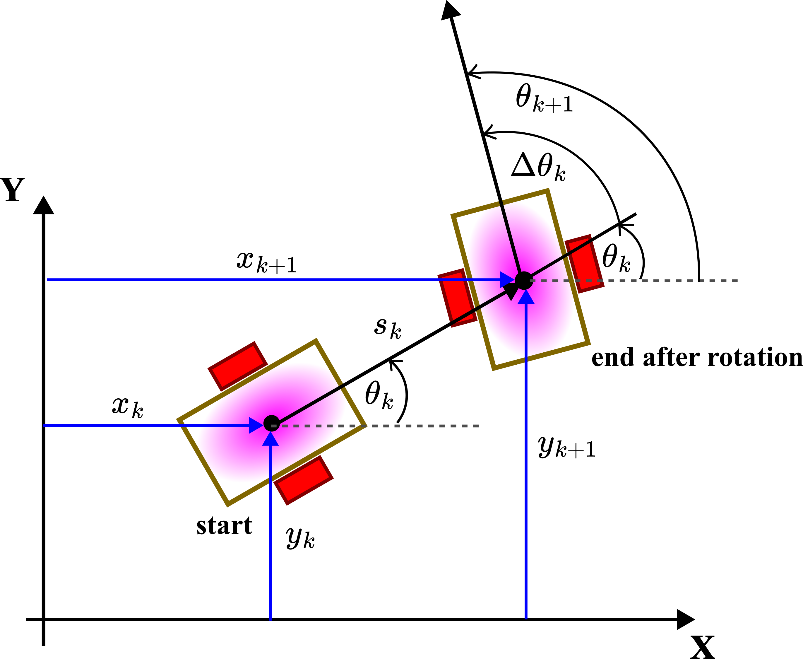
In the endpoint, we perform the rotation for the angle that is first introduced in equation (7). That is, the final orientation at the discrete-time instant is

(14)  

By combining (13) and (14), we obtain the final kinematics model of the mobile robot

(15)  

That is precisely the kinematics model (8) obtained by using discretization.

Important Remarks About the Derived Model

Here, for clarity, we repeat the derived model

(16)  

Usually, the traveled distance and the change of the angle are directly or indirectly measured by using sensors, such as wheel encoders, accelerometers, gyroscopes, compasses, etc. The process of obtaining these measurements is called odometry. Often in the robotics literature, you will see that and are used as known inputs. That is, although these quantities are actually measured outputs of the model, they are actually considered as the inputs! These inputs are measured at the discrete time instant . That is, at the end of the movement. This means that the model is written as follows

(17)  

where and are the measurements of and , respectively, that is

(18)