In our previous tutorial, which can be found here, we introduced the iterative policy evaluation algorithm for computing the state-value function. We also explained how to implement this algorithm in Python, and we tested the algorithm on the Frozen Lake Open AI Gym environment introduced in this post. The GitHub page with the codes developed in this tutorial is given here.
In this tutorial, we introduce a policy iteration algorithm. We explain how to implement this algorithm in Python and we explain how to solve the Frozen Lake problem by using this algorithm. Before reading this post, you should get yourself familiar with the following topics (links provided below):
- Frozen Lake environment and OpenAI Gym
- State value function and its Bellman equation
- The iterative policy evaluation algorithm
Motivation and Final Solution
Our goal is to solve the Frozen Lake problem. The Frozen Lake problem and its environment are explained in our previous post. This environment is illustrated in the figure below.

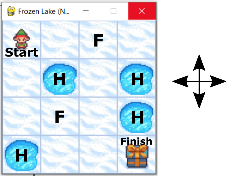
The goal is to reach “Finish” field starting from “Start” field. We can only perform the actions “UP”, “DOWN”, “LEFT”, and “RIGHT”. We have two types of fields: frozen field, denoted by “F”, and the hole field denoted by “H”. We can safely step on the frozen field. However, if we step on hole fields, we unsuccessfully end the game. The goal is to design a series of actions (“UP”,”DOWN”,”LEFT”, and “RIGHT”), such that we reach the finish the finish state by maximizing a reward function. In this post, we teach you how to solve this problem. The solution is shown in the figure below.

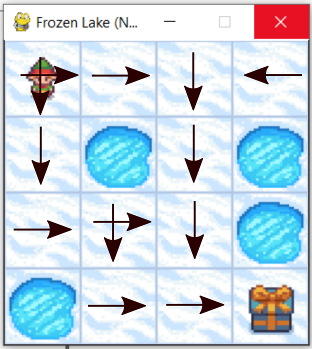
This solution is explained below.
Explanation of the Policy Iteration Algorithm
First, we need to introduce and explain the implementation of the policy iteration algorithm. The state value function is introduced and interpreted in our previous tutorial. The state value function has the following form, expressed by its Bellman equation:
(1) ![\begin{align*}v_{\pi}(s) & =E_{\pi}[G_{t}|S_{t}=s] \\v_{\pi}(s) & = \sum_{a} \pi(a|s) \sum_{s'}\sum_{r}p(s',r|s,a)[r+\gamma v_{\pi}(s')]\end{align*}](https://aleksandarhaber.com/wp-content/ql-cache/quicklatex.com-b73654d861dc49f013a4f2ca6f4a5898_l3.png "Rendered by QuickLaTeX.com")

where
![E_{\pi}[\cdot]](https://aleksandarhaber.com/wp-content/ql-cache/quicklatex.com-d8ca3e5443f3f8c37be84d5af753d326_l3.png "Rendered by QuickLaTeX.com")


-


-


In addition to the state value function (1), for the policy iteration algorithm, we also need an action-value function. The action value function is defined as follows:
(2) ![\begin{align*}q_{\pi}(s) & =E_{\pi}[G_{t}|S_{t}=s,A_{t}=a] \end{align*}](https://aleksandarhaber.com/wp-content/ql-cache/quicklatex.com-dc7fb11e0fbb4f4c132f77093b1b9b23_l3.png "Rendered by QuickLaTeX.com")

Here you should immediately notice the main difference between (1) and (2). The action value function is defined under the assumption that the agent takes an action
The Bellman equation for the action value function is
(3) ![\begin{align*}q_{\pi}(s)= \sum_{s'}\sum_{r}p(s',r|s,a)[r+\gamma v_{\pi}(s')]\end{align*}](https://aleksandarhaber.com/wp-content/ql-cache/quicklatex.com-f255c010355123813bfc98bd2a1359bf_l3.png "Rendered by QuickLaTeX.com")

In the sequel let us design an algorithm that will try to find an optimal policy that will maximize the state value function. That is, we want to find actions that will maximize the expected return from the state
(4) 

and we introduce the optimal action-value function
(5) 

Let the optimal policy that solves (4) and (5), be denoted by 

Next, we have that
(6) 

From the last equation, and by using a similar strategy to the strategy used to derive (3), we obtain the Bellman optimality equation for the state value function:
(7) ![\begin{align*}v_{*}(s)=\max_{a} \sum_{s'}\sum_{r}p(s',r|s,a)[r+\gamma v_{*}(s')]\end{align*}](https://aleksandarhaber.com/wp-content/ql-cache/quicklatex.com-5c926bc6a278fa6a1e45fb28d278e67a_l3.png "Rendered by QuickLaTeX.com")

The equations (3), (6), and (7) can give us a clue on how to determine an optimal policy. Let us say that we start our search for an optimal policy, with a certain policy 


(8) 

(9) ![\begin{align*}\text{action to take in state s} & = \underset{a}{\text{argmax}} \;\;\; \underbrace{\sum_{s'}\sum_{r}p(s',r|s,a)[r+\gamma v_{\pi_{0}}(s')]}_{q_{\pi_{0}}(s,a)}\end{align*}](https://aleksandarhaber.com/wp-content/ql-cache/quicklatex.com-242be27dec0842d7ae9ade15d57e6933_l3.png "Rendered by QuickLaTeX.com")

The solution of (9) actually defines an improved policy 


(10) ![\begin{align*} q_{\pi_{0}}(s,a) =\sum_{s'}\sum_{r}p(s',r|s,a)[r+\gamma v_{\pi_{0}}(s')] \end{align*}](https://aleksandarhaber.com/wp-content/ql-cache/quicklatex.com-5dab09f54adfddff4b670e0b2c7dcda9_l3.png "Rendered by QuickLaTeX.com")

for all possible actions
Next, for the newly computed policy 
(11) ![\begin{align*}\text{action to take in state s} & = \underbrace{\underset{a}{\text{argmax}} \;\;\; \sum_{s'}\sum_{r}p(s',r|s,a)[r+\gamma v_{\pi_{1}}(s')]}_{ q_{\pi_{1}}(s,a)}\end{align*}](https://aleksandarhaber.com/wp-content/ql-cache/quicklatex.com-e498ece64f711a77b6e48657f8a89a59_l3.png "Rendered by QuickLaTeX.com")

The solution of (11) defines a new policy 

POLICY ITERATION ALGORITHM:
Perform these two steps iteratively until convergence of the computed policy 
- Policy evaluation: For the policy

- Policy improvement: For the computed state-value function
(12)
![\begin{align*}& \text{action to take in state s} = \underset{a}{\text{argmax}} \;\;\; q_{\pi_{k}}(s,a) \\ & q_{\pi_{k}}(s,a)=\sum_{s'}\sum_{r}p(s',r|s,a)[r+\gamma v_{\pi_{k}}(s')] \end{align*}](https://aleksandarhaber.com/wp-content/ql-cache/quicklatex.com-7ef3bc2624854ea5259db00f84c9d0bd_l3.png "Rendered by QuickLaTeX.com")
The solution of (12) defines an improved policy


As mentioned previously this algorithm can be initialized with a complete random policy or with a policy obtained on the basis of some a priori knowledge about the environment.
Python Implementation
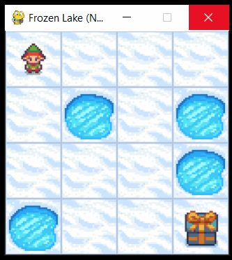
The GitHub page with the codes developed in this tutorial is given here. To test the policy iteration algorithm, we use the Frozen Lake environment explained in this tutorial. Here, we only provide a photo of the Frozen Lake environment, for more details see the tutorial. The Frozen Lake environment is shown in Fig. 3. below.

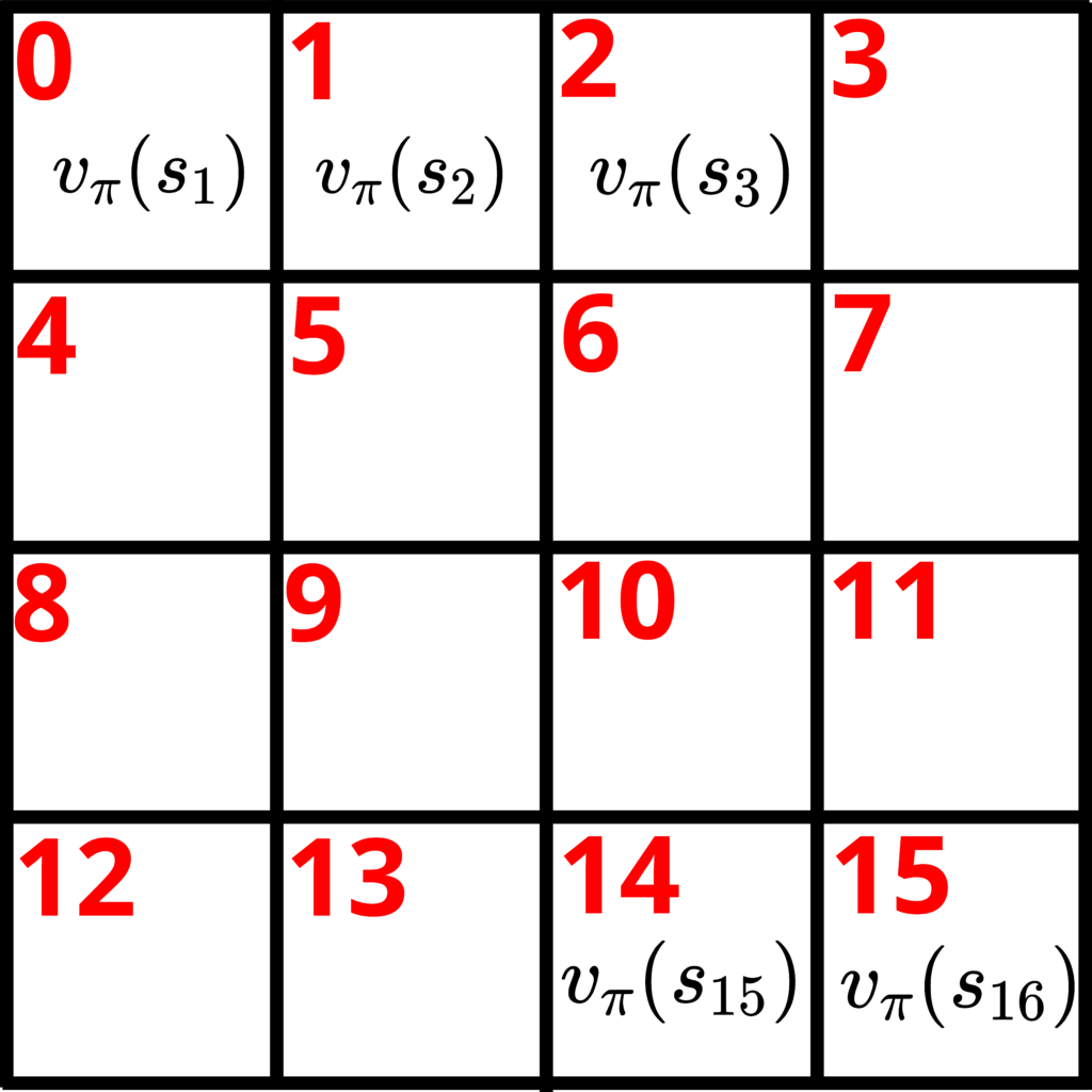
The states 


The first step is to define two functions. The first function will be used to implement the step 1 of the policy iteration algorithm. That is, this function will evaluate the policy or better to say, this function will compute the state-value function for a given policy. This function is actually developed in our previous tutorial, and here for brevity, we will not explain this function again. We will only briefly explain its inputs and outputs, and the general purpose. The function is given below.
##################
# this function computes the state value function by using the iterative policy evaluation algorithm
##################
# inputs:
##################
# env - environment
# valueFunctionVector - initial state value function vector
# policy - policy to be evaluated - this is a matrix with the dimensions (number of states)x(number of actions)
#        - p,q entry of this matrix is the probability of selection action q in state p
# discountRate - discount rate
# maxNumberOfIterations - max number of iterations of the iterative policy evaluation algorithm
# convergenceTolerance - convergence tolerance of the iterative policy evaluation algorithm
##################
# outputs:
##################
# valueFunctionVector - final value of the state value function vector

##################
def evaluatePolicy(env,valueFunctionVector,policy,discountRate,maxNumberOfIterations,convergenceTolerance):
    import numpy as np
    convergenceTrack=[]
    for iterations in range(maxNumberOfIterations):
        convergenceTrack.append(np.linalg.norm(valueFunctionVector,2))
        valueFunctionVectorNextIteration=np.zeros(env.observation_space.n)
        for state in env.P:
            outerSum=0
            for action in env.P[state]:
                innerSum=0
                for probability, nextState, reward, isTerminalState in env.P[state][action]:
                    #print(probability, nextState, reward, isTerminalState)
                    innerSum=innerSum+ probability*(reward+discountRate*valueFunctionVector[nextState])
                outerSum=outerSum+policy[state,action]*innerSum
            valueFunctionVectorNextIteration[state]=outerSum
        if(np.max(np.abs(valueFunctionVectorNextIteration-valueFunctionVector))<convergenceTolerance):
            valueFunctionVector=valueFunctionVectorNextIteration
            print('Iterative policy evaluation algorithm converged!')
            break
        valueFunctionVector=valueFunctionVectorNextIteration
    return valueFunctionVector
The first argument of this function, called “env” is the OpenAI Gym Frozen Lake environment. The second argument, called “valueFunctionVector” is the value function vector. It represents an initial value of the state-value function vector. This vector is iteratively updated by this function, and its value is returned. For the Frozen Lake environment, this vector has the following form
(13) 

The third argument, denoted by “policy” is a matrix defining the policy that needs to be evaluated. This matrix has this form
(14) 

where 


The second function implements the step 2 of the policy iteration algorithm. That is, this function is used to improve the policy. The function is given below.
##################
# this function computes an improved policy
##################
# inputs:
# env - environment
# valueFunctionVector - state value function vector that is previously computed
# numberActions - number of actions
# numberStates - number of states
# discountRate - discount rate

# outputs:
# improvedPolicy - improved policy
# qvaluesMatrix  - matrix containing computed action-value functions
#                - (p,q) entry of this matrix is the action value function computed at the state p and for the action q
# Note: qvaluesMatrix is just used for double check - it is actually not used lated on


##################

def improvePolicy(env,valueFunctionVector,numberActions,numberStates,discountRate):
    import numpy as np
    # this matrix will store the q-values (action value functions) for every state
    # this matrix is returned by the function
    qvaluesMatrix=np.zeros((numberStates,numberActions))
    # this is the improved policy
    # this matrix is returned by the function
    improvedPolicy=np.zeros((numberStates,numberActions))

    for stateIndex in range(numberStates):
        # computes a row of the qvaluesMatrix[stateIndex,:] for fixed stateIndex,
        # this loop iterates over the actions
        for actionIndex in range(numberActions):
            # computes the Bellman equation for the action value function
            for probability, nextState, reward, isTerminalState in env.P[stateIndex][actionIndex]:
                qvaluesMatrix[stateIndex,actionIndex]=qvaluesMatrix[stateIndex,actionIndex]+probability*(reward+discountRate*valueFunctionVector[nextState])

        # find the action indices that produce the highest values of action value functions
        bestActionIndex=np.where(qvaluesMatrix[stateIndex,:]==np.max(qvaluesMatrix[stateIndex,:]))

        # form the improved policy
        improvedPolicy[stateIndex,bestActionIndex]=1/np.size(bestActionIndex)
    return improvedPolicy,qvaluesMatrix
Let us explain this function. The first argument is “env” which is previously explained. The second argument is “valueFunctionVector” that is the state-value function vector defined in (13). The remaining 3 input arguments are self-explanatory. This function returns the matrix called “improvedPolicy”, This matrix has the form shown in Eq.(14). The second output argument, called “qvaluesMatrix” has the following form
(15) 

where 


(16) ![\begin{align*}\text{qvaluesMatrix}[0,:]=\begin{bmatrix} 0 & 0 & 0 & 1 \end{bmatrix}\end{align*}](https://aleksandarhaber.com/wp-content/ql-cache/quicklatex.com-ea3e7c00d7c9d5cc174d37ae7cd80223_l3.png "Rendered by QuickLaTeX.com")

On the other hand, it may happen that two values of 


(17) ![\begin{align*}\text{qvaluesMatrix}[0,:]=\begin{bmatrix} 0 & 0.5 & 0.5 & 0 \end{bmatrix}\end{align*}](https://aleksandarhaber.com/wp-content/ql-cache/quicklatex.com-3ed594aae1085b1e63ad801382ce2266_l3.png "Rendered by QuickLaTeX.com")

This means that we have a 50

import gym
import matplotlib.pyplot as plt
import seaborn as sns
import numpy as np
from functions import evaluatePolicy
from functions import improvePolicy

# create the environment
# this is a completely deterministic environment
env=gym.make('FrozenLake-v1', desc=None, map_name="4x4", is_slippery=False,render_mode="human")
# this is a completely stochastic environment - the algorithm will not work properly since the transition probabilities are equal -too much!
#env=gym.make("FrozenLake-v1", render_mode="human")
env.reset()
# render the environment
# uncomment this if you want to render the environment
env.render()
#
env.close()

# investigate the environment
# observation space - states
env.observation_space

env.action_space
# actions:
#0: LEFT
#1: DOWN
#2: RIGHT
#3: UP

##########################################################################
#           general parameters for the policy iteration
##########################################################################
# select the discount rate
discountRate=0.9
# number of states - determined by the Frozen Lake environment
stateNumber=16
# number of possible actions in every state - determined by the Frozen Lake environment
actionNumber=4
# maximal number of iterations of the policy iteration algorithm
maxNumberOfIterationsOfPolicyIteration=1000

# select an initial policy
# initial policy starts with a completely random policy
# that is, in every state, there is an equal probability of choosing a particular action
initialPolicy=(1/actionNumber)*np.ones((stateNumber,actionNumber))
##########################################################################
#           parameters of the iterative policy evaluation algorithm
##########################################################################
# initialize the value function vector
valueFunctionVectorInitial=np.zeros(env.observation_space.n)
# maximum number of iterations of the iterative policy evaluation algorithm
maxNumberOfIterationsOfIterativePolicyEvaluation=1000
# convergence tolerance
convergenceToleranceIterativePolicyEvaluation=10**(-6)
###########################################################################
###########################################################################

for iteration in range(maxNumberOfIterationsOfPolicyIteration):
    print("Iteration - {} - of policy iteration algorithm".format(iteration))
    if (iteration == 0):
        currentPolicy=initialPolicy
    valueFunctionVectorComputed =evaluatePolicy(env,valueFunctionVectorInitial,currentPolicy,discountRate,maxNumberOfIterationsOfIterativePolicyEvaluation,convergenceToleranceIterativePolicyEvaluation)
    improvedPolicy,qvaluesMatrix=improvePolicy(env,valueFunctionVectorComputed,actionNumber,stateNumber,discountRate)
    # if two policies are equal up to a certain "small" tolerance
    # then break the loop - our algorithm converged
    if np.allclose(currentPolicy,improvedPolicy):
        currentPolicy=improvedPolicy
        print("Policy iteration algorithm converged!")
        break
    currentPolicy=improvedPolicy
In the sequel, we only comment code lines that are not self-obvious. The code line 10 is used to is used to import the Frozen lake environment. Here it is very important to set the flag “is_slippery=False” . It is important to specify this flag to false since we want to ensure that the environment is deterministic. This means that the transition probabilities are 1. That is, 

currentPolicy=
array([[0.  , 0.5 , 0.5 , 0.  ],
       [0.  , 0.  , 1.  , 0.  ],
       [0.  , 1.  , 0.  , 0.  ],
       [1.  , 0.  , 0.  , 0.  ],
       [0.  , 1.  , 0.  , 0.  ],
       [0.25, 0.25, 0.25, 0.25],
       [0.  , 1.  , 0.  , 0.  ],
       [0.25, 0.25, 0.25, 0.25],
       [0.  , 0.  , 1.  , 0.  ],
       [0.  , 0.5 , 0.5 , 0.  ],
       [0.  , 1.  , 0.  , 0.  ],
       [0.25, 0.25, 0.25, 0.25],
       [0.25, 0.25, 0.25, 0.25],
       [0.  , 0.  , 1.  , 0.  ],
       [0.  , 0.  , 1.  , 0.  ],
       [0.25, 0.25, 0.25, 0.25]])
Taking into account that actions are encoded as follows:
#0: LEFT
#1: DOWN
#2: RIGHT
#3: UP
These actions are the columns of the matrix “currentPolicy”. This solution can graphically represented in the figure shown below. Consider the first row of the matrix currentPolicy. The first row of this matrix represents the actions we should take in the initial state 


