Clear Explanation of the Value Function and Its Bellman Equation – Reinforcement Learning Tutorial

In this reinforcement learning tutorial and in the accompanying YouTube video, we explain the meaning of the state value function and its Bellman equation. The motivation for creating this post and tutorial comes from the fact that the (state) value function and the corresponding Bellman equation play the main role in a number of reinforcement learning algorithms as well as in dynamic programming methods. On the other hand, in a number of books on reinforcement learning, the value function is only mathematically defined without providing the reader an intuitive understanding of its true meaning (if such a thing as “true meaning” exists at all since “true meaning” is definitely a philosophical term that has many interpretations). Usually, “heavy” probabilistic mathematics is involved in the definition, and students often cannot grasp the main idea behind this definition. This post aims at providing a clear understanding of the (state) value function.

Classical, “complex”, textbook definition of the value function and Bellman equation with Example

Here, we will follow the classical approach for defining the value function that can be found in many textbooks on reinforcement learning. This section uses the notation and partly follows the classical textbook on reinforcement learning

Sutton, R. S., & Barto, A. G. (2018). Reinforcement Learning: An Introduction. MIT Press.

As I mentioned previously, the proper understanding of definitions stated in this section, is often difficult for an average student and especially for students who are only interested in practical aspects of reinforcement learning. However, do not lose hope if you cannot understand the definitions stated in this section immediately! Hopefully, you will be able to understand them by the end of this tutorial (subsequent sections will be more “down to earth” when it comes to mathematics).

We have an agent that applies actions to a system or environment. The system can for example be a robotic manipulator or an autonomous driving vehicle. The agent can be a human or a control system. At a discrete time instant , our agent receives information about the environment state, denoted by . Then, on the basis of and its (control) policy, the agent selects an action and applies it to the system (environment). Then, at the time instant the environment responds to the action , and transitions to the next state , and our agent receives a numerical reward, denoted by , for this action. This process then continues, since the agent receives information about , and computes control actions .

This process generates a trajectory of states, actions, and rewards given below

(1)  

Here we should keep in mind that and are random variables. This is the main reason why they are denoted by capital letters. The particular values of these variables are denoted respectively by ,, and .

We illustrate the introduced concepts in this section with an example shown in figure 1.

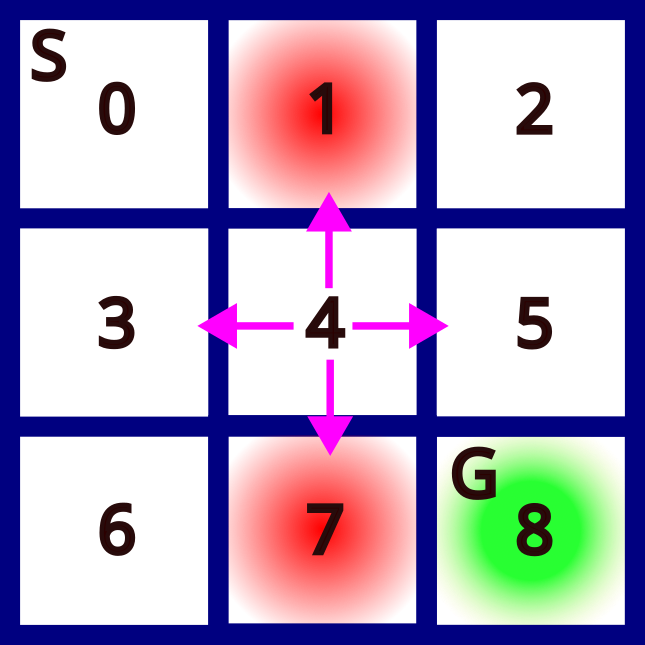
Figure 1 represents a grid world game. The starting state is the state “S” that is enumerated by . The goal is to reach the goal state denoted by “G”. At any field or state, we can perform the actions UP,DOWN, LEFT, and RIGHT. These actions are illustrated by magenta arrows in Fig. 1. By moving to certain fields we obtain a reward. For example, if we move to white fields 2,3,4,5, and 6, we obtain a reward of -1. If we arrive at the goal state G, we obtain a reward of 2. On the other hand, if we move to red fields 1 and 7, we obtain a reward of -10. These fields are the fields that we should avoid since they are not favorable. The rewards can for example be seen as fuel consumption or a penalty. Larger negative rewards mean more fuel consumption.

An episode is a series of actions, states, and rewards that start at the start state S and that end at the goal state G. An episode is shown in the figure below.

The actions are DOWN, LEFT, LEFT, DOWN. The states are . The obtained rewards are .

In the classical formulation of reinforcement learning problems, the environment response, obtained rewards, and agent actions are stochastic, that is, they are described by probabilities. The first important probability is the dynamics of the system or environment. This probability is also called the dynamics of the Markov Decision Process (MDP) and is defined as follows:

(2)  

In words, the dynamics of the MDP is the probability of reaching state and obtaining the reward at the time instant , if the system was in state at the time instant , and the agent applied the action at the time instant .

Another important definition is the definition of the state transition probability:

(3)  

In words, the state transition probability is the probability of reaching state at the time instant , if the system was in state at the time instant , and the agent applied the action at the time instant .

Here, immediately, a few things have to be noticed

1. The state at the previous time instant is denoted by (previous state). The state at the current time instant is denoted by (current state).
2. When the environment is in state and the agent applies the particular action , the environment will not necessarily transition to the same state! That is, there is a certain probability of reaching the particular state and obtaining a particular value of the reward . That is, the complete system composed of the agent and environment is stochastic or probabilistic!

Let us consider again the grid world game example introduced at the beginning of this section. Let us assume that we are at the state 0, and let us assume that in this state, the state transition probabilities for the action down are

(4)  

This means that although we perform action “DOWN” in state 0, this does not necessarily man that we will always go to the state 3 that is below the state 0. There is a probability of 0.6 that this will happen. For example, if we perform the action DOWN 100 times from state 0, approximately 60 times we will go to the state 3. Also, there is a probability of 0.2 that we will not move at all, that is that we will stay in the state 0. That is, the environment is stochastic or random!

The next concept we need to introduce is the concept of return. Let the sequence of the rewards obtained after the discrete-time step , be . Depending on the scenario, the return can be defined in several ways:

1. The undiscounted return for finite episodes is defined by
   
   

   (5)  

   
   where is the final step corresponding to the terminal state that ends an episode. An episode is a series of actions, rewards, and states that start from some state and that end up at a terminal state.
2. Discounted return for finite episodes
   
   

   (6)  

   
   where is the discount rate.
3. Discounted return for infinite episodes
   
   

   (7)  

For the explanation given in the sequel, it does not matter which definition we will use since these three definitions are not significantly changing the main ideas of the theoretical concepts that are developed in the sequel.

Here, a few important things should be kept in mind. Since the rewards are random variables, the return is also a random variable!

Also, from (7), we have

(8)  

Informally speaking, the goal of the reinforcement learning algorithm and its agent is to determine a series of actions that will maximize the return. However, we immediately arrive at one problem. Namely, since the return is a random variable, we cannot simply maximize the return. We actually need to maximize the expected return! This naturally leads us to the definition of the (state) value function. But before we introduce the state value function, we need to introduce the concept of the (control) policy.

The policy, denoted by is the probability of selecting the action when the current state is , that is

(9)  

Here again, one important thing should be noticed. In the general problem formulation, the (control) policies are not deterministic! That is, in a particular state at the time instant , there is a certain probability of selecting a particular action .

Let us go back to our grid world example once more. In state 4, the policy can for example be the following one

(10)  

These probabilities are illustrated in the figure 3 below.

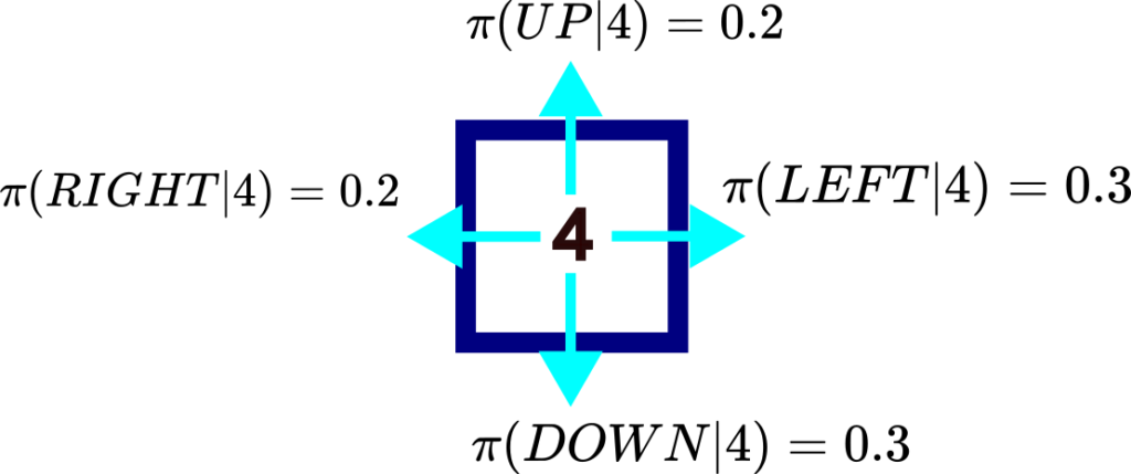
This policy makes sense since left and down actions have a higher probability since they lead us closer to the goal state G.

Now, we are finally ready to define the value function.

Definition of the value function: The value function of a particular state under the policy , denoted by , is the expectation of the return obtained by following the policy and starting from the state :

(11)  

here denotes the expected value of the random variable obtained under the assumption that the agent follows the policy . The value function of the terminal state is defined to be zero. Also, the value function is often called the state-value function for the policy .

A very important equation that enables us to iteratively compute the value function is the Bellman equation for the state value function .

Bellman equation for the state value function : Let be the state at the time instant , and be the state at the time instant . Then, it can be shown that

(12)  

where is the particular value of the reward obtained by reaching and is the state value function at .

Easy-to-understand derivation of the Bellman equation for the state value function is given here.

The Bellman equation for the state value function (12) looks very complex at a first glance. The goal of this post is to deconstruct the meaning of this equation and to help the interested reader to obtain a proper understanding of this equation, such that he or she can implement reinforcement learning algorithms that are based on this equation and on similar equations. Again, it is worth noting that this equation is the basis for a number of algorithms. Consequently, it is of paramount importance to properly understand this equation.

Meaning of the State Value Function

Let us now deconstruct the meaning of the state value function. We first need to obtain an intuitive understanding of mathematical expectations.

Understanding of expectations: Let us consider the game of throwing or rolling a six-sided die. Let us assume that the die is fair and that all sides are equally possible. We have six events or outcomes: , with equal probabilities .

The question is: “What is the expectation of throwing the die experiment?”

The expectation is defined by:

(13)  

On the other hand, the average or the mean of the outcomes is

(14)  

So the expectation is the same as the average in this case. So, why this is the case?

Let us imagine the following scenario. Let us throw the die 600 times. Since the dia is unbiased, we expect that approximately 100 times we will obtain 1, 100 times we will obtain 2, 100 times we will obtain 3, 100 times we will obtain 4, 100 times we will obtain 5, 100 times we will obtain 6. Let us compute the average:

(15)  

In the more general case, when some events are more likely, the expectation can be seen as a weighted average, where weights are proportional to the probability of occurrence of the event.

In other words, the expected value can be seen as a mean of numbers generated such that the number of times these a number appear matches the number’s probability of occurring. For example, let us say that our die is not fair. That is, the number 6 appears with 0.7 probability, and other numbers appear with a 0.06 probability. Then the expectation of the event of rolling a die is

(16)  

On the other hand, let us assume that we repeat this experiment 600 times. We should expect to see 1 approximately 36 times (probability of 0.06), 2 approximately 36 times, 3 approximately 36 times, 4 approximately 36 times , 5 approximately 36 times, and 6 approximately 420 times. Consequently, the average is

(17)  

Now that we understand the expectations, we can proceed further and explain the meaning of the value function.

Meaning of the value function- simple deterministic case:

We consider the environment shown in the figure below.

The start state is 0 and the end state is 4. Let us assume that in the states 1,2,3, and 4, we always obtain a constant reward of . Let us assume that

(18)  

Let us assume that we have a deterministic policy:

(19)  

That is, in any state, we always want to go left. Then, let us assume that the transition probability is also deterministic, that is

(20)  

That is, whenever we are in the state and we want to go left, we will actually go to the left state. Now, the question is what is our value function in the state then?

Our Bellman equation for the state is

(21)  

we only have a single action LEFT, and we only have a single next state , and we only can obtain a single reward when going from to and by taking the action “LEFT”, so we obtain

(22)  

On the other hand, by using the conditional probability theorem , we have

(23)  

Taking all these things into account, we obtain

(24)  

So the value function in the state is simply the reward obtained by going from the state to the next state plus the discounted value function in the next state. Now, let us consider the figure 4 once again, and let us compute the value functions in a backward manner:

(25)  

since is a terminal state, we have and consequently

(26)  

Similarly, we have

(27)  

We can see that the value functions at certain states are simply discounted returns! This is because the system is purely deterministic!

Meaning of the value function- grid world case:

Let us now go back to our grid world example that we show again in the figure below.

Let us again introduce the following assumptions

1. Rewards obtained at a certain destination state are deterministic, that is .
2. The policies for the actions UP,DOWN, LEFT, RIGHT have equal probability of for inner statew (state 4 ). That is,
   

   (28)  

   
   For other boundary states, the actions that will cause to hit the boundaries of the grid have zero probability (for example, actions UP and RIGHT in state 0 have a probability of 0).
3. The transition probabilities for every action in the state are equal. For example, this implies that for the state , we have
   

   (29)  

For simplicity, let us construct the state value function for the state 0. The Bellman equation for the state value function is

(30)  

Generally speaking, we have 4 actions. However, in state 0, we only have two possible actions LEFT, and DOWN. Consequently, a=LEFT, DOWN. Then, the next states are 1 and 3. That is, s’=1,3. Then, we have

(31)  

And, we only obtain a unique and deterministic reward in every destination state. Consequently, the sum over in (30) drops out

Consequently, the Bellman equation of the value function is

(32)  

The last equation can also be written as follows

(33)  

The Bellman equation of the value function has a graphical interpretation that is called a backup diagram. The backup diagram for the state is shown in the figure 6 below.

We start from the leaves. Every leaf node represents the term . By going upwards from the leaf node, we multiply this term by the corresponding probability . Then, the branch node sums the terms of the child nodes. Then, by going one level up, we multiply by , and finally at the top node we add these terms together.

On the other hand, we can construct the backup diagram as follows. Start from the state . From this state, we draw lines representing possible actions and denote policies for every action. This creates black nodes in the Fig. 6. Then, since the specific action from the state can lead to various states , we draw a line and a leaf node for every possible state, and denote the corresponding transition probability .

One very important observation can be made by analyzing the equation (33). Namely, this equation represents a weighted average of the terms . That is, the value function of represents a weighted average of the terms corresponding to all possible next states that can be reached starting from the state by following the policy .