Calibration and noise reduction of distance sensors (SHARP 2Y0A21 infrared sensors)

In this post, we consider the problems of calibration and noise reduction of distance sensors. In particular, we consider the class of InfraRed (IR) distance sensors produced by SHARP Corporation (2Y0A21, 0A41SK, etc). The methods presented in this post can be generalized to other sensor types, such as ultrasonic distance sensors, for example. A detailed video accompanying this video is given below.

The experiments are performed on the 2Y0A21 sensor, whose main specifications can be found here. According to the manufacturer specifications, the distance measurement range of this sensor is from 10 to 80 [cm]. However, this does not mean that the sensor cannot measure the distances from 0 to 10 [cm], as we will see later. The sensor photograph is given in Fig.1(a) below. The photograph of a MakerBeam sensor mount is shown in Fig.1(b).

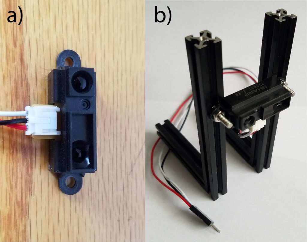
The sensor has three wires. The white wire is a signal wire. The red wire is a 5 [V] power wire, and the black wire is a ground wire. The connection diagram is shown in the figure below.

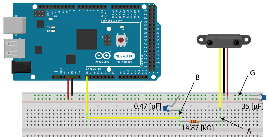
A few comments are in order. First, to stabilize the power supply line, we add a 35 [] bypass capacitor between the power (Vcc) and ground lines of the distance sensor. Without this capacitor, the measurements are extremely noisy. Then, we implement a low-pass filter using a 14.87 [] resistor and a 0.47 [] capacitor. The purpose of this filter is to additionally suppress high-frequency noise components. The cutoff frequency of this first-order low-pass filter is 143.1 [] or 22.8 []. This cutoff frequency is chosen on the basis of the fact that we are measuring distances of mechanical objects, which will not oscillate with high frequencies. For more details on implementing low-pass filters, see our previous post that can be found here.

The figure below shows the voltages of the signal wire without and with a low-pass filter. The voltage is measured using a Rigol oscilloscope.

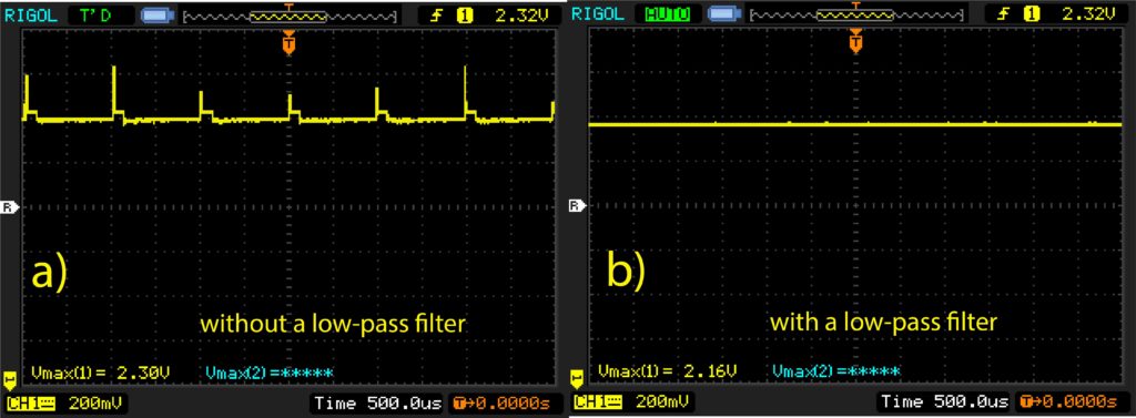
The plot (a) in Fig. 3 is generated by measuring the voltages between A-G points (see Figure 2). The plot (b) in Fig. 3 is generated by measuring the voltages between B-G points. From Fig. 3 we can observe that a simple RC circuit is able to significantly decrease the spurious measurement noise components and to smooth the signal.

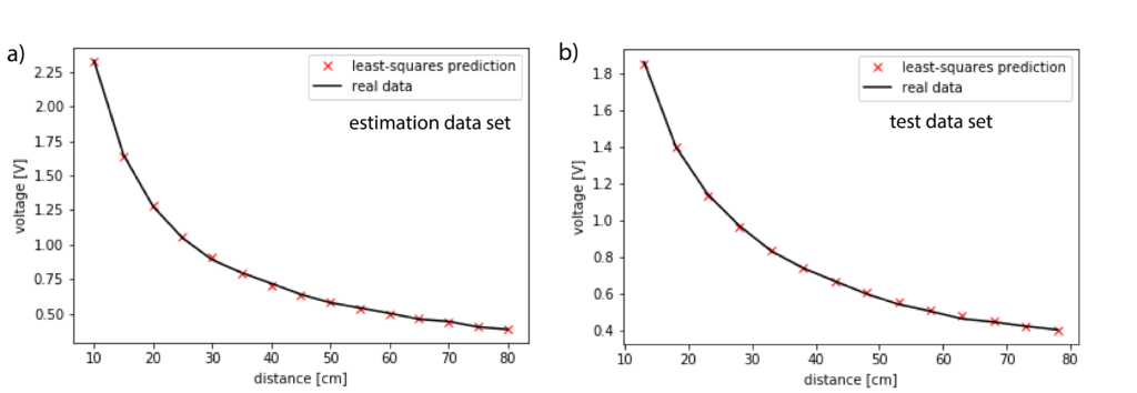
Next, we present a method for estimating function parameters relating the measured voltage and the distance. On the basis of our measurements (see the accompanying video), we obtain the following graph relating the distance and the voltages.

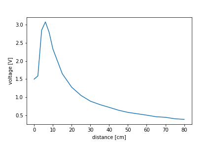
The shape of the observed curve is in accordance with the data reported by the manufacturer, for more details, see here. The voltage-distance function is not a bijection and consequently, its inverse does not exist. That is why we are only going to consider the part of the curve from 10 [cm] until 80 [cm]. In this range, the voltage-distance function can be approximated by the following function:

(1)  

where are real constants that need to be estimated, is the voltage, and is the distance. The above function is a nonlinear function and at first glance, it looks like that we would have to use a nonlinear least-squares method to estimate the constants and . However, using a simple trick, we can transform this equation into a form that can be used in an ordinary least-squares method. Namely, by taking the natural logarithm of both sides of equation \eqref{voltageDistanceGeneral}, we obtain

(2)  

By introducing the notation , , , and , we can write the last equation as follows:

(3)  

Next, let the , where is the -th voltage measurement at the distance . Correspondingly, we have . By grouping all measurements, we can use the following matrix notation to express all the voltage-distance measurements:

(4)  

The constants in the vector are estimated by solving the following least-squares problem:

(5)  

(6)  

Once this solution is computed, we can determine the constants and as follows:

(7)  

The estimated values are and . Once the constants are estimated, we can invert the function to obtain:

(8)  

We collect two data sets . The first data set is used to estimate the parameters using the above explained procedure. The second data set is used to test (validate) the estimation performance. The estimation and test performances are shown in figure below.

The Python code for estimating the coefficients and generating the plots is given below.

# -*- coding: utf-8 -*-
"""
the code for estimating the constants k1 and k2 in the equation:
    
voltage=k1*distance**(k2)

"""
import numpy as np
import matplotlib.pyplot as plt

# data for estimation
distances=np.array([0,2,4,6,8,10,15,20,25,30,35,40,45,50,55,60,65,70,75,80])
raw_measurements_total=(5/1024)*np.array([307.03, 325.07, 583.74, 630.45, 571.64, 477.43, 337.74, 261.53, 214.67, 182.46, 163.27, 147.54, 131.31, 119.07, 111.23, 103.44, 94.49, 91.23, 83.07, 79.54])
plt.plot(distances,raw_measurements_total)
plt.xlabel('distance [cm]')
plt.ylabel('voltage [V]')
plt.savefig('general_shape.png')
plt.show()

distances_trimed=distances[5:]
raw_measurements_total_trimed=raw_measurements_total[5:]

# validation data 
distances2=np.array([13,18,23,28,33,38,43,48,53,58,63,68,73,78])
raw_measurements2=(5/1024)*np.array([381.90, 286.85, 234.06, 198.68, 170.62, 151.54, 136.97, 122.71, 111.14, 103.46, 94.84, 91.34, 86.63, 82.75])

n=distances_trimed.shape[0]
y=np.zeros(shape=(n,1))
A=np.zeros(shape=(n,2))

for i in range(n):
    y[i,0]=np.log(raw_measurements_total_trimed[i])
    A[i,0]=1
    A[i,1]=np.log(distances_trimed[i])

# solution    
c=np.matmul(np.matmul(np.linalg.inv(np.matmul(A.T,A)),A.T),y)
k1=np.exp(c[0])
k2=c[1]

# test on the estimation data
raw_measurements_total_trimed_prediction=np.zeros(shape=(n,1))
for i in range(n):
    raw_measurements_total_trimed_prediction[i]=k1*distances_trimed[i]**(k2)

plt.plot(distances_trimed,raw_measurements_total_trimed_prediction,'xr',label='least-squares prediction')
plt.plot(distances_trimed,raw_measurements_total_trimed,'k',label='real data')
plt.xlabel('distance [cm]')
plt.ylabel('voltage [V]')
plt.legend()
plt.savefig('estimation_curve.png')
plt.show()

# test on the validation data 
n1=distances2.shape[0]
raw_measurements2_prediction=np.zeros(shape=(n1,1))
for i in range(n1):
    raw_measurements2_prediction[i]=k1*distances2[i]**(k2)
plt.plot(distances2,raw_measurements2_prediction,'xr',label='least-squares prediction')
plt.plot(distances2,raw_measurements2,'k',label='real data')
plt.xlabel('distance [cm]')
plt.ylabel('voltage [V]')
plt.legend()
plt.savefig('validation_curve.png')
plt.show()

The Arduino code for obtaining the measurement data is given below:

int analogPin = A0;
float sensorVal = 0;
float sensorVolt = 0;
float Vr=5.0;
float sum=0;

void setup() {
  Serial.begin(9600);
  
}

void loop() {

  sum=0;
  for (int i=0; i<100; i++)
  {
    sum=sum+float(analogRead(analogPin));  
  }
  sensorVal=sum/100;
  sensorVolt=sensorVal*Vr/1024;
  Serial.println(sensorVolt);
  delay(500);
}

The final Arduino code for measuring the distance on the basis of the estimation data is given below:

int analogPin = A0;
float sensorVal = 0;
float sensorVolt = 0;
float Vr=5.0;
float sum=0;
float k1=16.7647563;
float k2=-0.85803107;
float distance=0;
void setup() {
  Serial.begin(9600);
  
}

void loop() {

  sum=0;
  for (int i=0; i<100; i++)
  {
    sum=sum+float(analogRead(analogPin));  
  }
  sensorVal=sum/100;
  sensorVolt=sensorVal*Vr/1024;

  distance = pow(sensorVolt*(1/k1), 1/k2);
  Serial.println(distance);
  delay(500);
}