Fourier Series and Frequency Response

admin

6 years ago

In this post, we introduce frequency responses of linear systems and provide a brief introduction to Fourier series. Most importantly, we perform a real physical experiment of observing a frequency response of a resistor-capacitor (RC) circuit. A video about this post is given below. A YouTube video accompanying this post is given below. The video contains the frequency response measurement experiment.

Fourier Series

First, we provide a brief introduction to Fourier Series. Mr. Fourier, who was a French mathematician, claimed that any periodic function (even a periodic function with square corners!) can be used to be mathematically expressed as a sum of sinusoids! Sounds truly amazing.

So, let be a periodic function with the period of . According to Fourier, we can represent this function as follows

(1)

where

is the \textit{fundamental frequency},

is a complex coefficient,

is an imaginary unit. So how to find the Fourier Series expansion \eqref{FourierSeries} for a given function

. It can be shown that the coefficients are defined as follows:

(2)

Let us determine the Fouries series expansion for a periodic function shown in figure below.

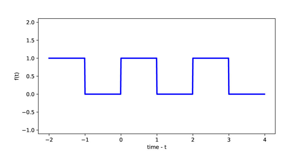
The period of this function is . This is a square wave function ( or a periodic pulse function) that is often encountered in signal analysis and control engineering. In its period This function can be formally expressed as follows:

(3)

where

is the function amplitude.
So let us apply the formula \eqref{fouriesCoefficients}

(4)

Next, we use the following trigonometric identities:

(5)

By using these identities in the previous expression, we obtain

(6)

Next, by using the Euler’s formula:

, we obtain

(7)

Now, we have to resolve possible indeterminate cases (when ). We notice that for , takes the form of . We can write:

(8)

where we used L’Hôpital’s rule to compute the limit (we can also use the limit of

to obtain the last result). On the other hand, we have:

(9)

By substituting the Euler’s formula, and by substituting the last expression as well as the expression for

given in \eqref{c0} in the expression \eqref{ FourierSeries }, we obtain

(10)

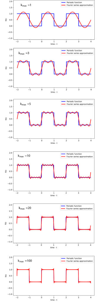
The following figure demonstrates the performance of the Fourier series expansion.

# -*- coding: utf-8 -*-
"""

Fourier series expansion - analytical

"""
import numpy as np
import matplotlib.pyplot as plt
import math
A=1
T=2

x=np.arange(-T,2*T,0.01)
y=np.zeros(shape=(x.shape[0],))
for i in range(x.shape[0]):
    if (x[i]<(-T/2)) or ((x[i]>0) and (x[i]<T/2)) or ((x[i]>T) and (x[i]<3*T/2)):
        y[i]=1
    

fig= plt.figure(figsize=(8,4))
plt.xlim(-2.5, 4.5)
plt.ylim(-0.2, 1.2)
plt.axis('equal')
plt.ylabel('f(t)')
plt.xlabel('time - t')
plt.plot(x,y,'b', linewidth=2.5, label='Periodic function')
plt.savefig('periodic_fuction.eps')


k_max=100
w0=2*math.pi/T
yapprox=[]

for i in range(x.shape[0]):
    sum=0
    for k in np.arange(1,k_max+1):
        sum=sum+A*((math.sin(k*math.pi/2))/(k*math.pi/2))*math.cos(k*w0*x[i]-k*math.pi/2)
    yapprox.append(sum+0.5*A)   
    

fig= plt.figure(figsize=(8,4))
plt.xlim(-2.5, 4.5)
plt.ylim(-0.2, 1.2)
plt.axis('equal')
plt.ylabel('f(t)')
plt.xlabel('time - t')
plt.plot(x,y,'b', linewidth=2.5,  label='Periodic function')
plt.plot(x,yapprox,'r', linewidth=2.5,  label='Fourier series approximation')
plt.legend()
plt.savefig('approximationk_100.eps')

Frequency Response

Consider a linear dynamical system S shown in Fig. 1.

Figure 1: A block diagram of a dynamical system.

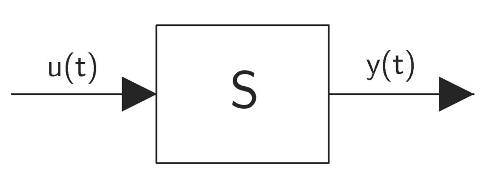
The system input is denoted by and the system output is . The input is an external signal affecting the system dynamics, and the output is a signal that we usually observe and whose dynamical behavior is of interest to us.

There are several ways of mathematically describing the relationship between the inputs and outputs. We can use differential equations to relate inputs and outputs. Differential equations can be used to argue about system stability and by solving them we can compute the system output for a given input. However, in many situations, we would like to have a simpler representation of the system behavior, that can be more useful from an engineering standpoint.

Frequency response is such a system representation. First, we will motivate the need for frequency response functions.

We know that (almost) every (periodic) function can be represented as a sum of harmonic functions (sin() and cos() functions). This follows from the Fourier series expansion. For example, consider a periodic ramp function:

(11)

and where the period is

. Its Fourier series expansion is:

(12)

Motivated by this, let us write the input function

as follows:

(13)

where

is the angular frequency and

is a real constant. Since the system is linear, the sytem response to the input

(14)

where

is the system response to the harmonic function

. So, the system response can be computed by summing the system responses to basic cos() functions.

This motivates us to consider the following problem. What is the system response when the input function is

? The answer is that it is again a cos() function, with unaltered angular frequency and with phase and amplitude changes that depend on the frequency. How can we show this?

First of all, we know that the system response can be computed as a convolution of an impulse response and the input:

(15)

where

is the impulse response. The impulse response is the system response for the impulse function

(Dirac delta function). This function is zero everywhere except at 0 where it has an infinite value. Furthermore, its integral from minus infinity to plus infinity is 1. From the engineering point of view, this function is obtained by exciting the system with a low duration and a high-intensity pulse. Let us assume that the input is given as follows:

(16)

where

is generally a complex number. Substituting \eqref{ inputU} in \eqref{convolution1}, we obtain:

(17)

where the term

(18)

is the system transfer function. Notice that the system transfter function is the Laplace transformation of the impulse response function. Let us now use \eqref{transfer1} to compute the system response to a cos() function. Using the Euler’s relation, we can write:

(19)

where

is the imaginary unit and

(20)

Since the system is linear, the reponse to the input

in \eqref{cosEuler} is a sum of the responses to

and

. Let us compute the response to

. Taking into account that

and using \eqref{transfer1}, we can write:

(21)

On the other hand,

is a complex number and it can be represented in the polar form:

, where

is the magnitude and

is the phase. Using this transformation, \eqref{y1First} can be expressed as follows:

(22)

For

, we can write:

(23)

Since

, we have:

(24)

Finally, we have:

(25)

From the Euler’s relation, it follows that the second term in the last expression is equal to

. That is,

(26)

To conclude, if the system input is

, the output function

. The conclusion is that the system does not alter the frequncy, but it generally speaking alters the amplitude and the phase.

The frequency response is characterized by the following two functions:

(27)

The first one in \eqref{frequencyResponse1} is the magnitude response. It tells us the amplification of the amplitude of the input signal. The second one in \eqref{frequencyResponse2} is the phase response. The phase response gives us information about the delay of the output signal with respect to the input signal.

In the sequel, we derive a frequency response of an RC circuit, and we present experimental results of observing the response for several frequency values. The RC circuit is shown in Fig. 2.

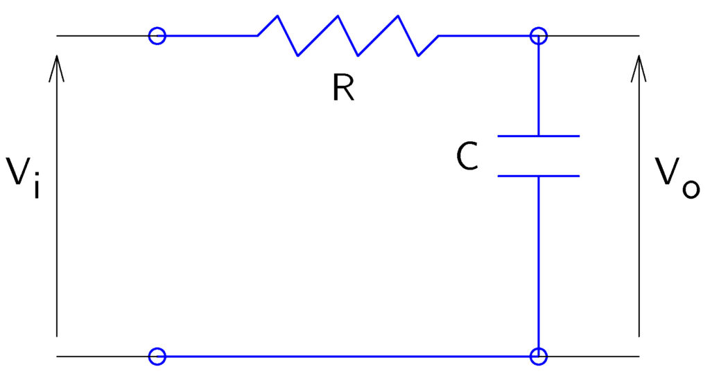
A differential equation describing the relation between the input () and output () voltages is

(28)

where

is a time constant. Taking the Laplace transform of the last equation we obtain:

(29)

where

and

are the Laplace transforms of

and

, respectively, and

. For the computation of the transfer function, we assume that the initial conditions are zero. Consequently, we obtain:

(30)

For , we have

(31)

From the last equation we conclude:

(32)

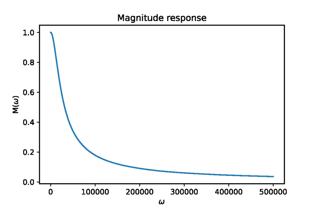
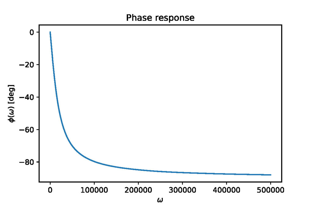
Next, we simulate the frequency response. The Python code is given below:

<pre class="wp-block-syntaxhighlighter-code">import numpy as np
import matplotlib.pyplot as plt

R=550
C=100*10**(-9)
T=R*C

w=0.5*np.arange(1000000)
M=(np.sqrt(1+(T*w)**(2)))**(-1)
phi=-np.arctan(T*w)*(180/np.pi)

plt.plot(w,M)
plt.title('Magnitude response')
plt.xlabel('<img src="https://aleksandarhaber.com/wp-content/ql-cache/quicklatex.com-707fcec15e450815730425a6607a1858_l3.png" class="ql-img-inline-formula quicklatex-auto-format" alt="&#92;&#111;&#109;&#101;&#103;&#97;" title="Rendered by QuickLaTeX.com" height="8" width="11" style="vertical-align: 0px;"/>')
plt.ylabel('M(<img src="https://aleksandarhaber.com/wp-content/ql-cache/quicklatex.com-707fcec15e450815730425a6607a1858_l3.png" class="ql-img-inline-formula quicklatex-auto-format" alt="&#92;&#111;&#109;&#101;&#103;&#97;" title="Rendered by QuickLaTeX.com" height="8" width="11" style="vertical-align: 0px;"/>)')
plt.savefig('magnitude.eps')
plt.show()


plt.plot(w, phi)
plt.title('Phase response')
plt.xlabel('<img src="https://aleksandarhaber.com/wp-content/ql-cache/quicklatex.com-707fcec15e450815730425a6607a1858_l3.png" class="ql-img-inline-formula quicklatex-auto-format" alt="&#92;&#111;&#109;&#101;&#103;&#97;" title="Rendered by QuickLaTeX.com" height="8" width="11" style="vertical-align: 0px;"/>')
plt.ylabel('<img src="https://aleksandarhaber.com/wp-content/ql-cache/quicklatex.com-5b2be26c0c1341f54b29baddda771346_l3.png" class="ql-img-inline-formula quicklatex-auto-format" alt="&#92;&#112;&#104;&#105;" title="Rendered by QuickLaTeX.com" height="16" width="11" style="vertical-align: -4px;"/>(<img src="https://aleksandarhaber.com/wp-content/ql-cache/quicklatex.com-707fcec15e450815730425a6607a1858_l3.png" class="ql-img-inline-formula quicklatex-auto-format" alt="&#92;&#111;&#109;&#101;&#103;&#97;" title="Rendered by QuickLaTeX.com" height="8" width="11" style="vertical-align: 0px;"/>) [deg]')
plt.savefig('phase.eps')
plt.show()</pre>

Here are the magnitude and phase responses plots:

Another important concept we need to introduce is the concept of the cutoff frequency. The cutoff frequency is usually defined as the frequency at which the magnitude response is equal to . That is, at this frequency the amplitude of the output signal is times the amplitude of the input signal. Let us see what is the cutoff frequency of the RC circuit. We have

(33)

From here, we have:

(34)

The experimental results of measuring certain points of an RC circuit are given in the Figure below. The results are generated for and .

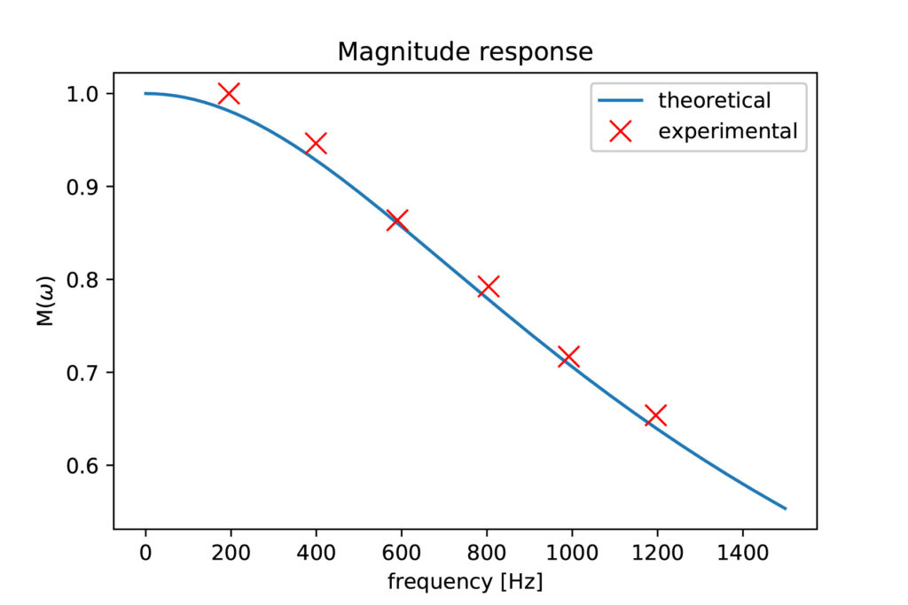
The code for generating these plots is given below and for more details see the video.

<pre class="wp-block-syntaxhighlighter-code">import numpy as np
import matplotlib.pyplot as plt
import math
R=330
C=484*10**(-9)
T=R*C
freq_theoretical=1*np.arange(1500)
M=1/(np.sqrt(1+(T*(2*np.pi*freq_theoretical))**(2)))
phi=-np.arctan(T*(2*np.pi*freq_theoretical))*(180/np.pi)

cutoff=1/(R*C*2*math.pi)

frequency = np.array([195, 399, 590,  804, 992, 1196])
vout_max   = np.array([4.56, 4.24, 3.8, 3.36, 3.04,  2.72])
vin_max  = np.array([4.56, 4.48,   4.40, 4.24, 4.24,  4.16])
M_measured= vout_max/vin_max


plt.plot(freq_theoretical,M,label='theoretical')
plt.plot(frequency,M_measured,'rx',markersize=10,label='experimental')
plt.title('Magnitude response')
plt.xlabel('frequency [Hz]')
plt.ylabel('M(<img src="https://aleksandarhaber.com/wp-content/ql-cache/quicklatex.com-707fcec15e450815730425a6607a1858_l3.png" class="ql-img-inline-formula quicklatex-auto-format" alt="&#92;&#111;&#109;&#101;&#103;&#97;" title="Rendered by QuickLaTeX.com" height="8" width="11" style="vertical-align: 0px;"/>)')
plt.legend()
plt.savefig('magnitude1.eps')
plt.show()
</pre>