In this control engineering, control theory, and machine learning, we present a Model Predictive Control (MPC) tutorial. First, we explain how to formulate the problem and how to solve it. Finally, we explain how to implement the MPC algorithm in C++ by using the Eigen C++ matrix library. In this tutorial, we consider MPC for linear dynamical systems and we consider the unconstrained case. Also, since this is the first part of a series of tutorials, we assume that the state vector is completely known. In future tutorials, we will develop MPC algorithms when the state is not known. That is, we will integrate an observer with the MPC algorithms. In the first part of this tutorial series, we explained how to implement the MPC algorithm in Python. The first part can be found here. The GitHub page with C++ code files is given here. The YouTube tutorial is given below.

Here is the motivation for creating this video tutorial. Namely, most control engineering classes and teachers focus on MATLAB/Simulink without providing the students and engineers with the necessary knowledge on how to implement in C++ or Python. That is, students rarely have the opportunity to learn real-life implementation of control/estimation algorithms. There is a huge gap between what people learn in undergraduate and graduate programs with what the industry needs and wants. Also, graduate students studying control are focused too much on advanced mathematics and theorem proofs and they rarely have a chance to learn C++ and how to implement algorithms. On the other hand, computer science students have good coding skills. However, they often do not study advanced mathematical concepts necessary to understand control theory and engineering. That is, there is a huge knowledge gap that students need to fill. To be a successful model-based control engineer who will be able to tackle advanced problems one needs to be proficient in control theory and math on one side and in coding on the other side. The free tutorials I am creating aim to fill this knowledge gap.
How to Cite This Document:
“Model Predictive Control (MPC) Tutorial 2: Unconstrained Solution for Linear Systems and Implementation in C++ from Scratch by Using Eigen C++ Library”. Technical Report, Number 3, Aleksandar Haber, (2023), Publisher: www.aleksandarhaber.com, Link: https://aleksandarhaber.com/model-predictive-control-mpc-tutorial-2-unconstrained-solution-for-linear-systems-and-implementation-in-c-from-scratch-by-using-eigen-c-library/
When citing this tutorial and the report, include the link.
Model Predictive Control Formulation
We consider the linear system
(1) 

where 


In our problem formulation 

Next, we need to introduce the following notation which is also illustrated in the figure below.

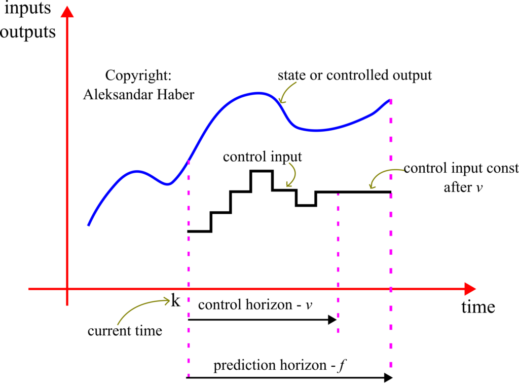
- The length of the prediction horizon is denoted by

- The length of the control horizon is denoted by


The goal of the model predictive controller is to determine a set of control inputs 


Let us assume that we are currently at the time instant 


(2) 

Then, by using the last equation, we can write the state and output predictions for the time instant 
(3) 

By using the same principle, for the time instant 
(4) 

The last equation can be written in the compact form
(5) 

By continuing with this procedure until the time index
(6) 

The index
(7) 

This is a constraint that we impose on our controller. By using this equation, we have for the time index 

(8) 

By using the same procedure and by shifting the time index, we obtain the prediction for the final step
(9) 

The last equation can be written compactly
(10) 

where
(11) 

In the general case, we introduce the following notation for 
(12) 

By combining all the prediction equations in a single equation, we obtain
(13) 

where 


The last equation can be written compactly as follows
(14) 

where
(15) 

The model predictive control problem can be formulated as follows. The goal is to track a reference output trajectory. Let these desired outputs be denoted by
(16) 

where the superscript “d” means that the outputs are desired outputs. Let the vector 

(17) 

A natural way of formulating the model predictive control problem is to determine the vector of control inputs 

(18) 

where 

The part of the cost function that will penalize the inputs has the following form
(19) 

where 


(20) 

The last expression can be written compactly as
(21) 

where
(22) 

and where
(23) 

where
(24) 

The matrix 

Next, we introduce the part of the cost function that corresponds to the tracking error:
(25) 

By introducing
(26) 

where 


(27) 

where
(28) 

This part of the cost function penalizes the difference between the desired trajectory and the controlled trajectory. Let us analyze the part of the cost function (27). Since it is assumed that the state vector 

(29) 

By substituting (23) and (27) in (29), we obtain
(30) 

Next, we need to minimize the cost function (30). To do that, let us write
(31) 

Next, we need to minimize the expression 


(32) 

Then, by using these two equations, we can differentiate all the terms in (31):
(33) 

(34) 

(35) 

(36) 

(37) 

By using (33)-(37), we can compute the derivative of the cost function
(38) 

To find the minimum of the cost function with respect to
(39) 

From where we obtain
(40) 

(41) 

From the last equation, we obtain the solution of the model predictive control problem:
(42) 

It can be shown that this is the solution that actually minimizes the cost function 

(43) 

We only need the first entry, that is 


The derived model predictive control algorithm can be summarized as follows.
STEP 1: At the time instant 

STEP 2: Extract the first entry of this solution
STEP 3: Wait for the system to respond and obtain the state measurement
Model for Testing the Model Predictive Controller
We consider a mass-spring damper system as a test case for the model predictive controller. The state-space model of this system is derived in our previous tutorial which can be found here. The model is shown in the figure below.

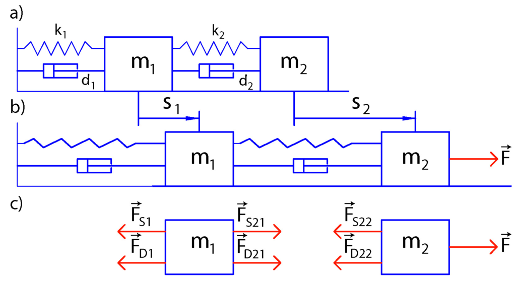
The state-space model has the following form:
(44) 

(45) 

The next step is to transform the state-space model (44)-(45) in the discrete-time domain. Due to its simplicity and good stability properties, we use the Backward Euler method to perform the discretization. This method approximates the state derivative as follows
(46) 

where 


(47) 

where 


(48) 

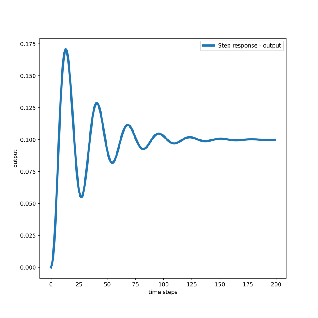
The step response of the system is shown below (the codes are given in the first tutorial part).

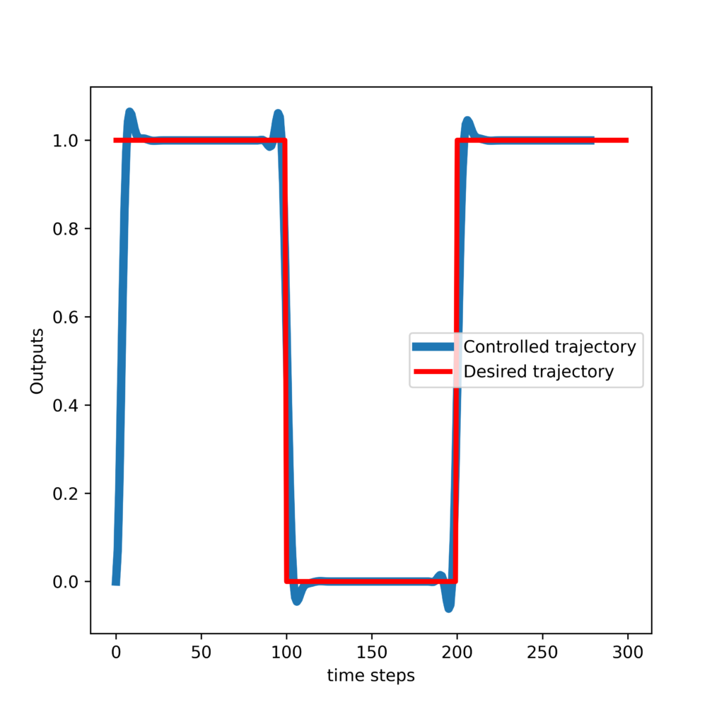
Numerical Results
In this section, we present the numerical results. The C++ codes are given in the next section. We select a reference (desired) trajectory that is a pulse function. The figure below shows the reference trajectory and the response of the model predictive controller.
The figure below shows the computed control inputs.

C++ Implementation of Model Predictive Control Algorithm
The code files presented in this section are available on the GitHub page whose link is given here. The following class implements the Model Predictive Control algorithm in C++. For a detailed explanation of the code, see the YouTube video tutorial at the beginning of this page. First, we give the header file of the class. The code presented below should be saved in the file “ModelPredictiveController.h”.
/*
Model Predictive Control implementation in C++
Author:Aleksandar Haber
Date: September 2023

We implemented a Model Predictive Control (MPC) algorithm in C++ by using the Eigen C++ Matrix library
The description of the MPC algorithm is given in this tutorial:

https://aleksandarhaber.com/model-predictive-control-mpc-tutorial-1-unconstrained-formulation-derivation-and-implementation-in-python-from-scratch/

This is the header file of the Model Predictive Controller class
*/
#ifndef MODELPREDICTIVECONTROLLER_H
#define MODELPREDICTIVECONTROLLER_H

#include<string>
#include<Eigen/Dense>
using namespace Eigen;
using namespace std;


class ModelPredictiveController{
    public:
        // default constructor - edit this later
        ModelPredictiveController();

        /*
        This constructor will initialize all the private variables,
        and it will construct the lifted system matrices O and M,
        as well as the control gain matrix necessary to compute the control inputs
        */
        // this is the constructor that we use
        // Ainput, Binput, Cinput - A,B,C system matrices
        // fInput - prediction horizon
        // vInput - control horizon
        // W3input, W4input - weighting matrices, see the tutorial
        // x0Input - x0 initial state of the system
        // desiredControlTrajectoryTotalInput - total desired input trajectory

        ModelPredictiveController(MatrixXd Ainput, MatrixXd Binput, MatrixXd Cinput,
                     unsigned int fInput, unsigned int vInput,
                     MatrixXd W3input, MatrixXd W4input,
                     MatrixXd x0Input, MatrixXd desiredControlTrajectoryTotalInput);

        // this function is used to propagate the dynamics and to compute the solution of the MPC problem
        void computeControlInputs();

        // this function is used to save the variables as "csv" files
        // desiredControlTrajectoryTotalFile - name of the file used to store the trajectory
        // inputsFile  - name of the file used to store the computed inputs
        // statesFile  - name of the file used to store the state trajectory
        // outputsFile  - name of the file used to store the computed outputs - this is the controlled output
        // Ofile        - name of the file used to store the O lifted matrix - you can use this for diagonostics
        // Mfile        - name of the file used to store the M lifted matrix - you can use this for diagonostics
        void ModelPredictiveController::saveData(string desiredControlTrajectoryTotalFile, string inputsFile,
							string statesFile, string outputsFile,string OFile, string MFile) const;

    private:


        // this variable is used to track the current time step k of the controller
        // it is incremented in the function computeControlInputs()
        unsigned int k;

        // m - input dimension, n- state dimension, r-output dimension
        unsigned int m,n,r;

        // MatrixXd is an Eigen typdef for Matrix<double, Dynamic, Dynamic>
	    MatrixXd A,B,C,Q; // system matrices
        MatrixXd W3,W4;   // weighting matrices
	    MatrixXd x0;      // initial state
        MatrixXd desiredControlTrajectoryTotal; // total desired trajectory
        unsigned int f,v; // f- prediction horizon, v - control horizon


        // we store the state vectors of the controlled state trajectory
        MatrixXd states;

        // we store the computed inputs
        MatrixXd inputs;

        // we store the output vectors of the controlled state trajectory
        MatrixXd outputs;

        // lifted system matrices O and M, computed by the constructor
        MatrixXd O;
        MatrixXd M;

        // control gain matrix, computed by constructor
        MatrixXd gainMatrix;

};

#endif
Then, we give the implementation file of the class. The code presented below should be saved in the file “ModelPredictiveController.cpp”.
/*
Model Predictive Control implementation in C++
Author:Aleksandar Haber
Date: September 2023

We implemented a Model Predictive Control (MPC) algorithm in C++ by using the Eigen C++ Matrix library
The description of the MPC algorithm is given in this tutorial:

https://aleksandarhaber.com/model-predictive-control-mpc-tutorial-1-unconstrained-formulation-derivation-and-implementation-in-python-from-scratch/

This is the implementation file of the Model Predictive Controller class
*/

#include <iostream>
#include<tuple>
#include<string>
#include<fstream>
#include<vector>
#include<Eigen/Dense>
#include "ModelPredictiveController.h"

using namespace Eigen;
using namespace std;

// edit this default constructor later
ModelPredictiveController::ModelPredictiveController()
{
}


        /*
        This constructor will initialize all the private variables,
        and it will construct the lifted system matrices O and M,
        as well as the control gain matrix necessary to compute the control inputs
        */
        // this is the constructor that we use
        // Ainput, Binput, Cinput - A,B,C system matrices
        // fInput - prediction horizon
        // vInput - control horizon
        // W3input, W4input - weighting matrices, see the tutorial
        // x0Input - x0 initial state of the system
        // desiredControlTrajectoryTotalInput - total desired input trajectory

ModelPredictiveController::ModelPredictiveController(
    MatrixXd Ainput, MatrixXd Binput, MatrixXd Cinput,
    unsigned int fInput, unsigned int vInput,
    MatrixXd W3input, MatrixXd W4input,
    MatrixXd x0Input, MatrixXd desiredControlTrajectoryTotalInput)
{

    A=Ainput; B=Binput; C=Cinput;
    f=fInput; v=vInput;
    W3=W3input; W4=W4input;
    x0=x0Input; desiredControlTrajectoryTotal=desiredControlTrajectoryTotalInput;

    // m - input dimension, n- state dimension, r-output dimension
    // extract the appropriate dimensions
    n = A.rows();   m = B.cols(); r = C.rows();

    // this variable is used to track the current time step k of the controller
    k=0;

    // the trajectory is a column matrix
    unsigned int maxSimulationSamples = desiredControlTrajectoryTotal.rows() - f;

    // we store the state vectors of the controlled state trajectory
    states.resize(n, maxSimulationSamples);
    states.setZero();
    states.col(0)=x0;

    // we store the computed inputs
    inputs.resize(m, maxSimulationSamples-1);
    inputs.setZero();

    // we store the output vectors of the controlled state trajectory
    outputs.resize(r, maxSimulationSamples-1);
    outputs.setZero();


    // we form the lifted system matrices O and M and the gain control matrix

    // form the lifted O matrix
    O.resize(f*r,n);
    O.setZero();

    // this matrix is used to store the powers of the matrix A for forming the O matrix
    MatrixXd powA;
    powA.resize(n,n);

    for (int i=0; i<f;i++)
    {
        if (i == 0)
        {
            powA=A;
        }
        else
        {
            powA=powA*A;
        }

            O(seq(i*r,(i+1)*r-1),all)=C*powA;
    }

    // form the lifted M matrix
    M.resize(f*r,v*m);
    M.setZero();

    MatrixXd In;
    In= MatrixXd::Identity(n,n);

    MatrixXd sumLast;
    sumLast.resize(n,n);
    sumLast.setZero();

    for (int i=0; i<f;i++)
    {
        // until the control horizon
        if(i<v)
        {
            for (int j=0; j<i+1;j++)
            {
                if (j==0)
                {
                    powA=In;
                }
                else
                {
                    powA=powA*A;


                }
                M(seq(i*r,(i+1)*r-1),seq((i-j)*m,(i-j+1)*m-1))=C*powA*B;
            }
        }
        // from the control horizon until the prediction horizon
        else
        {
            for(int j=0;j<v;j++)
            {
                if (j==0)
                {
                        sumLast.setZero();
                        for (int s=0;s<i+v+2;s++)
                        {
                            if (s == 0)
                            {
                                powA=In;
                            }
                            else
                            {
                                powA=powA*A;
                            }
                            sumLast=sumLast+powA;
                        }
                        M(seq(i*r,(i+1)*r-1),seq((v-1)*m,(v)*m-1))=C*sumLast*B;


                }
                else
                {

                    powA=powA*A;
                    M(seq(i*r,(i+1)*r-1),seq((v-1-j)*m,(v-j)*m-1))=C*powA*B;


                }

            }

        }
    }

    MatrixXd tmp;
    tmp.resize(v*m,v*m);

    tmp=M.transpose()*W4*M+W3;
    gainMatrix=(tmp.inverse())*(M.transpose())*W4;

}


// this function propagates the dynamics
// and computes the control inputs by solving the model predictive control problem
void ModelPredictiveController::computeControlInputs()
{

    // # extract the segment of the desired control trajectory
    MatrixXd desiredControlTrajectory;
    desiredControlTrajectory=desiredControlTrajectoryTotal(seq(k,k+f-1),all);

    //# compute the vector s
    MatrixXd vectorS;
    vectorS=desiredControlTrajectory-O*states.col(k);

    //# compute the control sequence
    MatrixXd inputSequenceComputed;
    inputSequenceComputed=gainMatrix*vectorS;
    // extract the first entry that is applied to the system
    inputs.col(k)=inputSequenceComputed(seq(0,m-1),all);

    // propagate the dynamics
    states.col(k+1)=A*states.col(k)+B*inputs.col(k);
    outputs.col(k)=C*states.col(k);

    //increment the index
    k=k+1;

}


  // this function is used to save the variables as "csv" files
        // desiredControlTrajectoryTotalFile - name of the file used to store the trajectory
        // inputsFile  - name of the file used to store the computed inputs
        // statesFile  - name of the file used to store the state trajectory
        // outputsFile  - name of the file used to store the computed outputs - this is the controlled output
        // Ofile        - name of the file used to store the O lifted matrix - you can use this for diagonostics
        // Mfile        - name of the file used to store the M lifted matrix - you can use this for diagonostics

void ModelPredictiveController::saveData(string desiredControlTrajectoryTotalFile, string inputsFile,
							string statesFile, string outputsFile, string OFile, string MFile) const
{
	const static IOFormat CSVFormat(FullPrecision, DontAlignCols, ", ", "\n");

	ofstream file1(desiredControlTrajectoryTotalFile);
	if (file1.is_open())
	{
		file1 << desiredControlTrajectoryTotal.format(CSVFormat);

		file1.close();
	}

	ofstream file2(inputsFile);
	if (file2.is_open())
	{
		file2 << inputs.format(CSVFormat);
		file2.close();
	}

	ofstream file3(statesFile);
	if (file3.is_open())
	{
		file3 << states.format(CSVFormat);
		file3.close();
	}

	ofstream file4(outputsFile);
	if (file4.is_open())
	{
		file4 << outputs.format(CSVFormat);
		file4.close();
	}

    ofstream file5(OFile);
	if (file5.is_open())
	{
		file5 << O.format(CSVFormat);
		file5.close();
	}


ofstream file6(MFile);
	if (file6.is_open())
	{
		file6 << M.format(CSVFormat);
		file6.close();
	}


}
Finally, the driver code for the class is given below.
/*
Model Predictive Control implementation in C++
Author:Aleksandar Haber
Date: September 2023

We implemented a Model Predictive Control (MPC) algorithm in C++ by using the Eigen C++ Matrix library
The description of the MPC algorithm is given in this tutorial:

https://aleksandarhaber.com/model-predictive-control-mpc-tutorial-1-unconstrained-formulation-derivation-and-implementation-in-python-from-scratch/

This is the driver code that explains how to use the Model Predictive Controller class
and that solves the MPC problem
*/

#include <iostream>
#include<Eigen/Dense>

#include "ModelPredictiveController.h"
#include "ModelPredictiveController.cpp"

using namespace Eigen;
using namespace std;


int main()
{

//###############################################################################
//#  Define the MPC algorithm parameters
//###############################################################################

// prediction horizon
unsigned int f=20;
// control horizon
unsigned int v=18;

//###############################################################################
//# end of MPC parameter definitions
//###############################################################################


//###############################################################################
//# Define the model - continious time
//###############################################################################

//# masses, spring and damper constants
double m1=2  ; double m2=2   ; double k1=100  ; double k2=200 ; double d1=1  ; double d2=5;
//# define the continuous-time system matrices and initial condition

    Matrix <double,4,4> Ac {{0, 1, 0, 0},
                            {-(k1+k2)/m1 ,  -(d1+d2)/m1 , k2/m1 , d2/m1},
                            {0 , 0 ,  0 , 1},
                            {k2/m2,  d2/m2, -k2/m2, -d2/m2}};
    Matrix <double,4,1> Bc {{0},{0},{0},{1/m2}};
    Matrix <double,1,4> Cc {{1,0,0,0}};

    Matrix <double,4,1> x0 {{0},{0},{0},{0}};

//  m- number of inputs
//  r - number of outputs
//  n - state dimension
  unsigned int n = Ac.rows();  unsigned int m = Bc.cols(); unsigned int r = Cc.rows();


//###############################################################################
//# end of model definition
//###############################################################################

//###############################################################################
//# discretize the model
//###############################################################################

//# discretization constant
double sampling=0.05;

// # model discretization
// identity matrix
MatrixXd In;
In= MatrixXd::Identity(n,n);

MatrixXd A;
MatrixXd B;
MatrixXd C;
A.resize(n,n);
B.resize(n,m);
C.resize(r,n);
A=(In-sampling*Ac).inverse();
B=A*sampling*Bc;
C=Cc;

//###############################################################################
//# end of discretize the model
//###############################################################################

//###############################################################################
//# form the weighting matrices
//###############################################################################

//# W1 matrix
MatrixXd W1;
W1.resize(v*m,v*m);
W1.setZero();

MatrixXd Im;
Im= MatrixXd::Identity(m,m);

for (int i=0; i<v;i++)
{
  if (i==0)
  {
     W1(seq(i*m,(i+1)*m-1),seq(i*m,(i+1)*m-1))=Im;
  }
  else
  {
     W1(seq(i*m,(i+1)*m-1),seq(i*m,(i+1)*m-1))=Im;
     W1(seq(i*m,(i+1)*m-1),seq((i-1)*m,(i)*m-1))=-Im;
  }

}


//# W2 matrix
double Q0=0.0000000011;
double Qother=0.0001;

MatrixXd W2;
W2.resize(v*m,v*m);
W2.setZero();

for (int i=0; i<v; i++)
{
  if (i==0)
  {
    // this is for multivariable
    //W2(seq(i*m,(i+1)*m-1),seq(i*m,(i+1)*m-1))=Q0;

    W2(i*m,i*m)=Q0;
  }
  else
  {
    // this is for multivariable
    //W2(seq(i*m,(i+1)*m-1),seq(i*m,(i+1)*m-1))=Qother;
    W2(i*m,i*m)=Qother;

  }


}

MatrixXd W3;
W3=(W1.transpose())*W2*W1;


MatrixXd W4;
W4.resize(f*r,f*r);
W4.setZero();

// # in the general case, this constant should be a matrix
double predWeight=10;

for (int i=0; i<f;i++)
{
   //this is for multivariable
  //W4(seq(i*r,(i+1)*r-1),seq(i*r,(i+1)*r-1))=predWeight;
  W4(i*r,i*r)=predWeight;
}


//###############################################################################
//# end of form the weighting matrices
//###############################################################################

//###############################################################################
//# Define the reference trajectory
//###############################################################################

unsigned int timeSteps=300;

//# pulse trajectory

MatrixXd desiredTrajectory;
desiredTrajectory.resize(timeSteps,1);
desiredTrajectory.setZero();

MatrixXd tmp1;
tmp1=MatrixXd::Ones(100,1);

desiredTrajectory(seq(0,100-1),all)=tmp1;

desiredTrajectory(seq(200,timeSteps-1),all)=tmp1;

//###############################################################################
//# end of definition of the reference trajectory
//###############################################################################

//###############################################################################
//# Run the MPC algorithm
//###############################################################################


// create the MPC object
ModelPredictiveController  mpc(A, B, C,
    f, v,W3,W4,x0,desiredTrajectory);

// this is the main control loop
for (int index1=0; index1<timeSteps-f-1; index1++)
{
  mpc.computeControlInputs();
}

// save the computed vectors and matrices
// saveData(string desiredControlTrajectoryTotalFile, string inputsFile,
// 							string statesFile, string outputsFile)
mpc.saveData("trajectory.csv", "computedInputs.csv",
                            "states.csv", "outputs.csv","Omatrix.csv","Mmatrix.csv");

cout<<"MPC simulation completed and data saved!"<<endl;
return 0;

}
By running this driver code, several comma-separated value (csv) files will be generated. These files store the computed inputs, outputs, and states, as well as the reference (desired) trajectory and the lifted system matrices 


# -*- coding: utf-8 -*-
"""
/*
Model Predictive Control implementation in C++
Author:Aleksandar Haber
Date: September 2023

We implemented a Model Predictive Control (MPC) algorithm in C++ by using the Eigen C++ Matrix library
The description of the MPC algorithm is given in this tutorial:

https://aleksandarhaber.com/model-predictive-control-mpc-tutorial-1-unconstrained-formulation-derivation-and-implementation-in-python-from-scratch/

This is the Python file used to visualize the results
and to save the graphs

This file will load the saved matrices and vectors.
After that, it will generate the graphs
*/
"""

import numpy as np
import matplotlib.pyplot as plt

# Load the matrices and vectors from csv files
# computed control inputs
cppInputs = np.loadtxt("computedInputs.csv", delimiter=",")
# controlled state trajectory
cppStates = np.loadtxt("states.csv", delimiter=",")
# computed outputs
cppOutputs= np.loadtxt("outputs.csv", delimiter=",")
# reference (desired) trajectory
cppTrajectory= np.loadtxt("trajectory.csv", delimiter=",")
# lifted O matrix
Omatrix=np.loadtxt("Omatrix.csv", delimiter=",")
# lifted M matrix
Mmatrix=np.loadtxt("Mmatrix.csv", delimiter=",")

# plot the results

plt.figure(figsize=(6,6))
plt.plot(cppOutputs,linewidth=5, label='Controlled trajectory')
plt.plot(cppTrajectory,'r', linewidth=3, label='Desired trajectory')
plt.xlabel('time steps')
plt.ylabel('Outputs')
plt.legend()
plt.savefig('controlledOutputsPulseCpp.png',dpi=600)
plt.show()


plt.figure(figsize=(6,6))
plt.plot(cppInputs,linewidth=4, label='Computed inputs')
plt.xlabel('time steps')
plt.ylabel('Input')
plt.legend()
plt.savefig('inputsPulseCpp.png',dpi=600)
plt.show()