In this control engineering, control theory, and machine learning, we present a Model Predictive Control (MPC) tutorial. First, we explain how to formulate the problem and how to solve it. Finally, we explain how to implement the MPC algorithm in Python. In this tutorial, we consider MPC for linear dynamical systems and we consider the unconstrained case. Also, since this is the first part of a series of tutorials, we assume that the state vector is completely known. In future tutorials, we will develop MPC algorithms when the state is not known. That is, we will integrate an observer with the MPC algorithms. Also, in future tutorials, we will consider the constrained MPC algorithms and MPC for nonlinear systems. The C++ implementation of the MPC algorithm is given here. The GitHub page with the developed code files is given here. The YouTube page accompanying this tutorial is given below.

The main challenge was how to make a tutorial that was easy for beginners without going immediately into nonlinear and complex optimization worlds, where students immediately get lost and immediately give up on studying MPC. This comment also applies to modern control theory. A number of control scientists publishing papers in Automatica/IEEE TAC simply do not put effort into explaining things such that everyone can understand the basic concepts. There is a trend to make the control theory as complex as possible and as a pure math discipline. I think that was not the vision of the founders of control theory, who were actually engineers solving real-life problems. In fact, control theory is super applicable and relatively easy. The only issue is that one has to conquer math to be able to apply it. Consequently, I start with the MPC formulation for linear systems and I try to stick as much as possible to basic linear algebra.
We explain how to formulate a least-squares cost function, and how to minimize it. The solution can be expressed in a closed form as a solution of a weighted least-squares problem. The input constraints can be implicitly handled by properly selecting weighting matrices. We then explain how to implement this algorithm in Python from scratch and in a disciplined and clean manner (by using Python classes). We test the algorithm on a classical system consisting of two objects connected by springs and dampers. In the second part of this tutorial series, we will consider constrained linear systems. In the third part, we will consider nonlinear smooth systems (the most general formulation). After we complete the Python model predictive control tutorials, we will start a new tutorial series on how to implement the algorithm in C++ by using the Eigen Library.
How to Cite This Document:
“Model Predictive Control (MPC) Tutorial 1: Unconstrained Formulation, Derivation, and Implementation in Python from Scratch”. Technical Report, Number 2, Aleksandar Haber, (2023), Publisher: www.aleksandarhaber.com, Link: https://aleksandarhaber.com/model-predictive-control-mpc-tutorial-1-unconstrained-formulation-derivation-and-implementation-in-python-from-scratch/
When citing this tutorial and the report, include the link.
Model Predictive Control Formulation
We consider the linear system
(1) 

where 


In our problem formulation 

Next, we need to introduce the following notation which is also illustrated in the figure below.

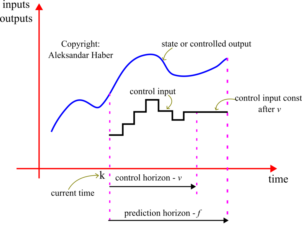
- The length of the prediction horizon is denoted by

- The length of the control horizon is denoted by


The goal of the model predictive controller is to determine a set of control inputs 


Let us assume that we are currently at the time instant 


(2) 

Then, by using the last equation, we can write the state and output predictions for the time instant 
(3) 

By using the same principle, for the time instant 
(4) 

The last equation can be written in the compact form
(5) 

By continuing with this procedure until the time index
(6) 

The index
(7) 

This is a constraint that we impose on our controller. By using this equation, we have for the time index 

(8) 

By using the same procedure and by shifting the time index, we obtain the prediction for the final step
(9) 

The last equation can be written compactly
(10) 

where
(11) 

In the general case, we introduce the following notation for 
(12) 

By combining all the prediction equations in a single equation, we obtain
(13) 

where 


The last equation can be written compactly as follows
(14) 

where
(15) 

The model predictive control problem can be formulated as follows. The goal is to track a reference output trajectory. Let these desired outputs be denoted by
(16) 

where the superscript “d” means that the outputs are desired outputs. Let the vector 

(17) 

A natural way of formulating the model predictive control problem is to determine the vector of control inputs 

(18) 

where 

The part of the cost function that will penalize the inputs has the following form
(19) 

where 


(20) 

The last expression can be written compactly as
(21) 

where
(22) 

and where
(23) 

where
(24) 

The matrix 

Next, we introduce the part of the cost function that corresponds to the tracking error:
(25) 

By introducing
(26) 

where 


(27) 

where
(28) 

This part of the cost function penalizes the difference between the desired trajectory and the controlled trajectory. Let us analyze the part of the cost function (27). Since it is assumed that the state vector 

(29) 

By substituting (23) and (27) in (29), we obtain
(30) 

Next, we need to minimize the cost function (30). To do that, let us write
(31) 

Next, we need to minimize the expression 


(32) 

Then, by using these two equations, we can differentiate all the terms in (31):
(33) 

(34) 

(35) 

(36) 

(37) 

By using (33)-(37), we can compute the derivative of the cost function
(38) 

To find the minimum of the cost function with respect to
(39) 

From where we obtain
(40) 

(41) 

From the last equation, we obtain the solution of the model predictive control problem:
(42) 

It can be shown that this is the solution that actually minimizes the cost function 

(43) 

We only need the first entry, that is 


The derived model predictive control algorithm can be summarized as follows.
STEP 1: At the time instant 

STEP 2: Extract the first entry of this solution
STEP 3: Wait for the system to respond and obtain the state measurement
Model for Testing the Model Predictive Controller
We consider a mass-spring damper system as a test case for the model predictive controller. The state-space model of this system is derived in our previous tutorial which can be found here. The model is shown in the figure below.

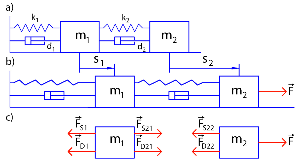
The state-space model has the following form:
(44) 

(45) 

The next step is to transform the state-space model (44)-(45) in the discrete-time domain. Due to its simplicity and good stability properties, we use the Backward Euler method to perform the discretization. This method approximates the state derivative as follows
(46) 

where 


(47) 

where 


(48) 

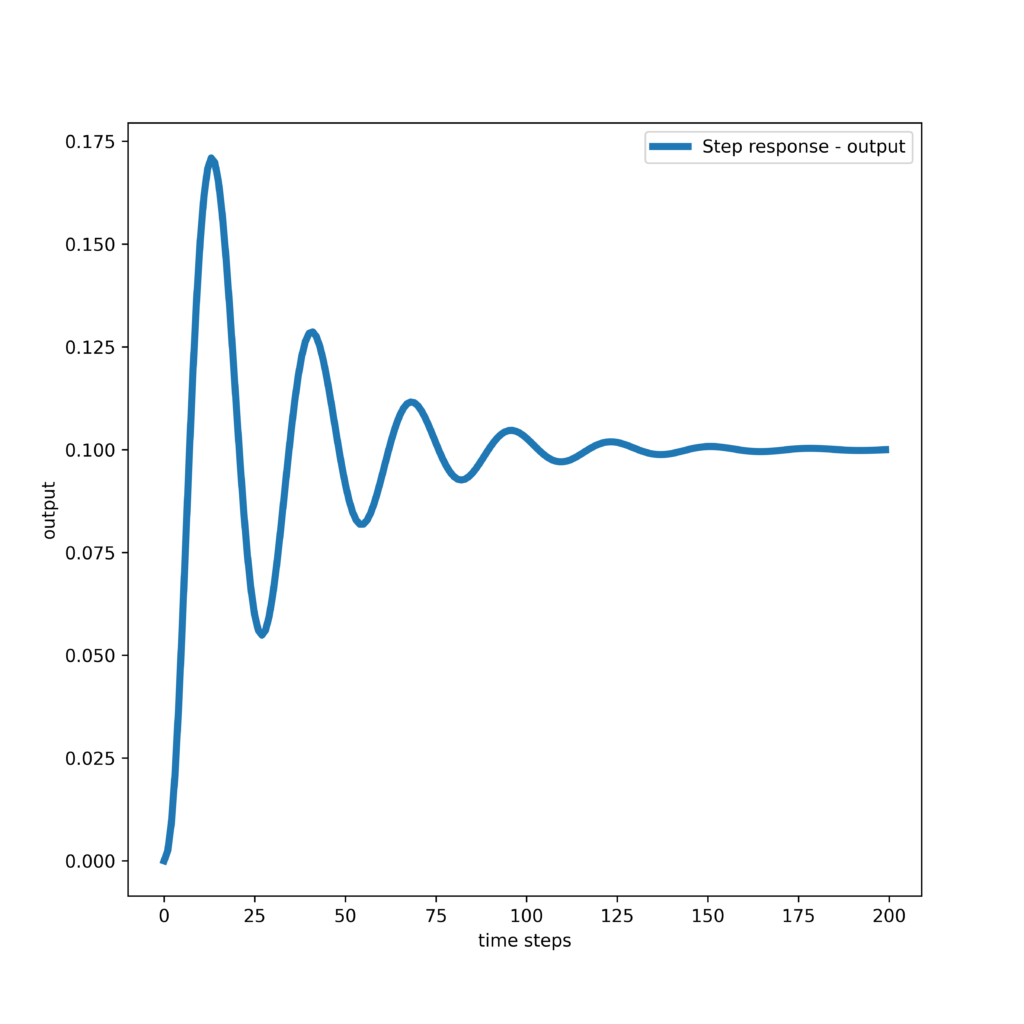
The step response of the system is shown below (the codes are given in the section on Python implementation).

Numerical Tests of Applying the Model Predictive Controller
Here, we present numerical tests of applying the model predictive controller. The Python codes used to generate these results are presented in the next section.
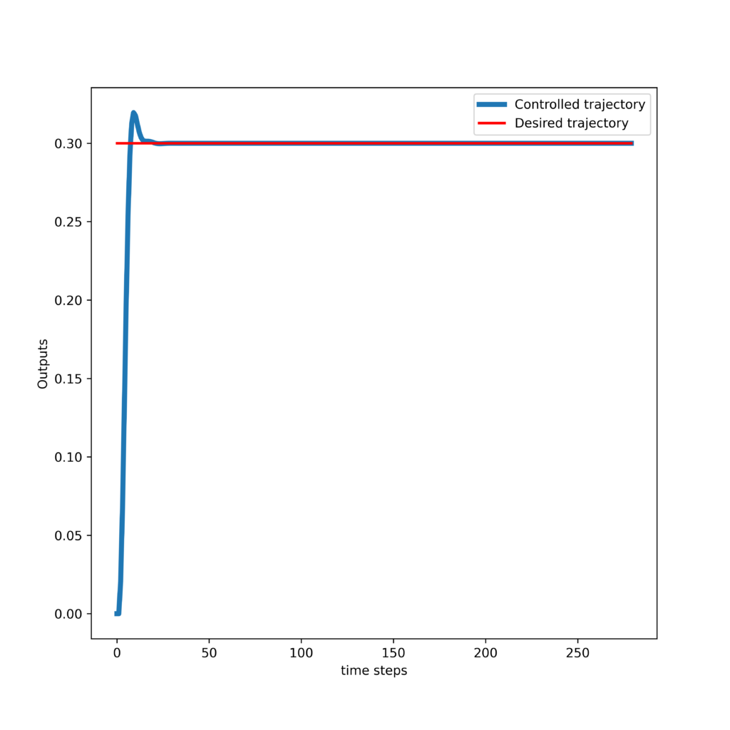
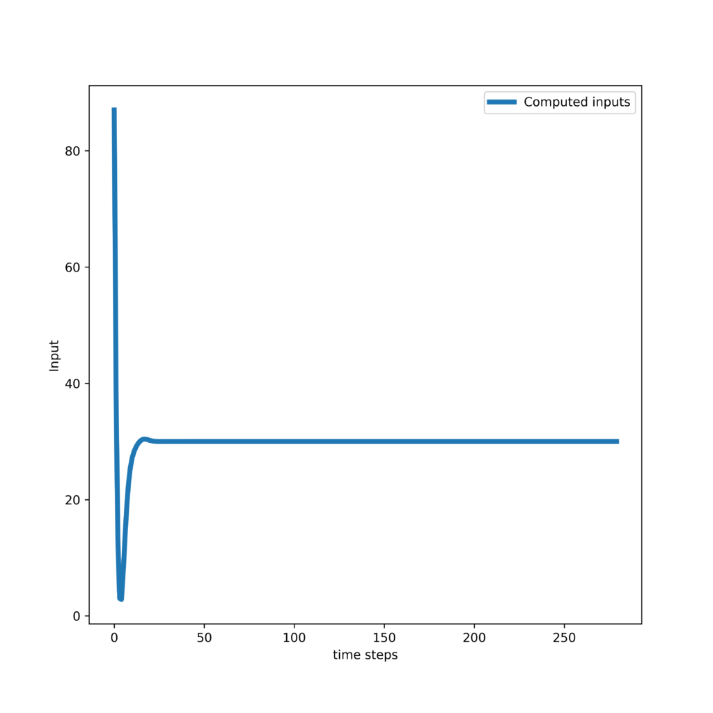
First, we present the results obtained by tracking a step trajectory. The response of the controller and control inputs are shown in the two graphs given below.
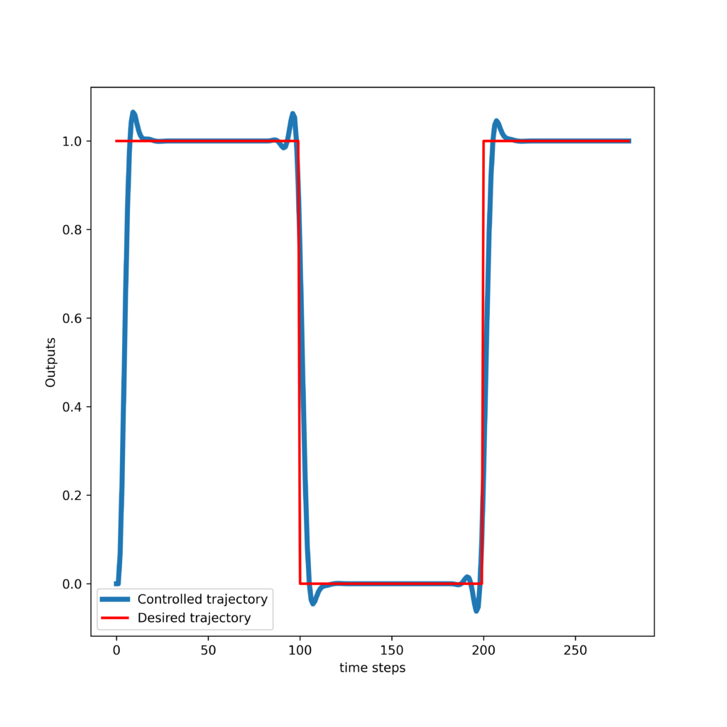
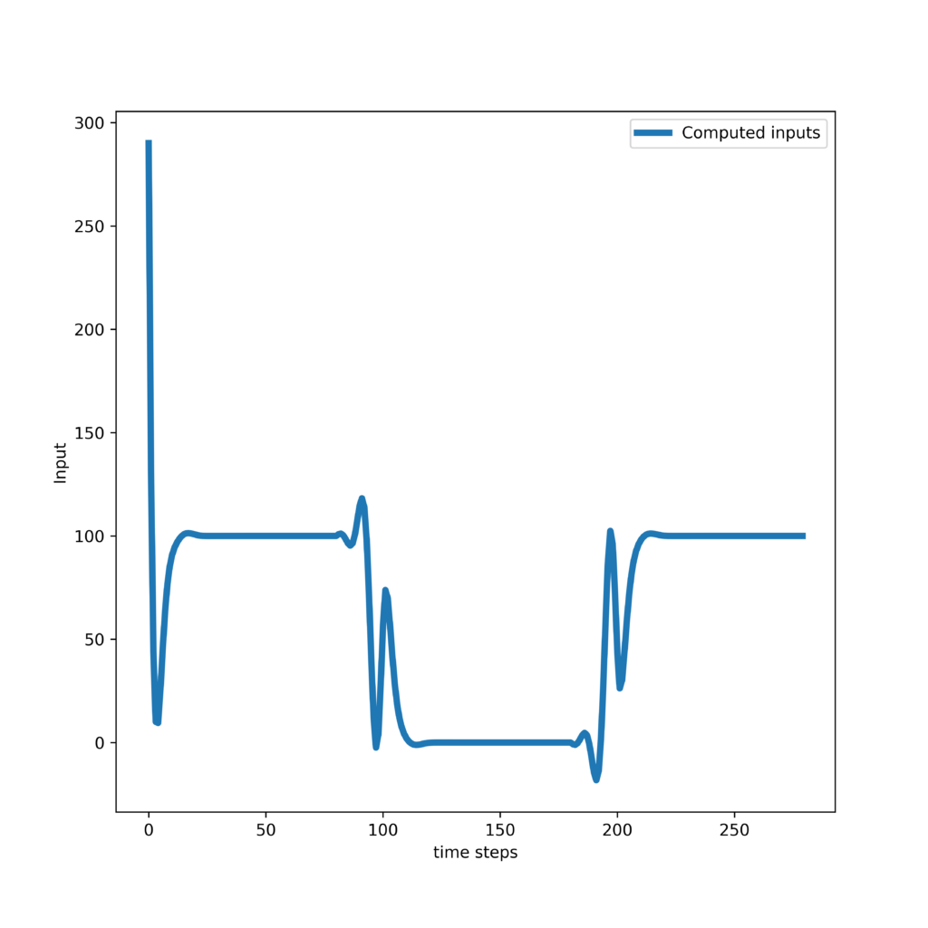
Secondly, we present the results obtained by tracking a pulse trajectory. The response of the controller and control inputs are shown in the two graphs given below.
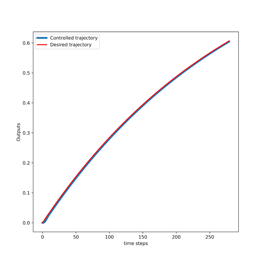
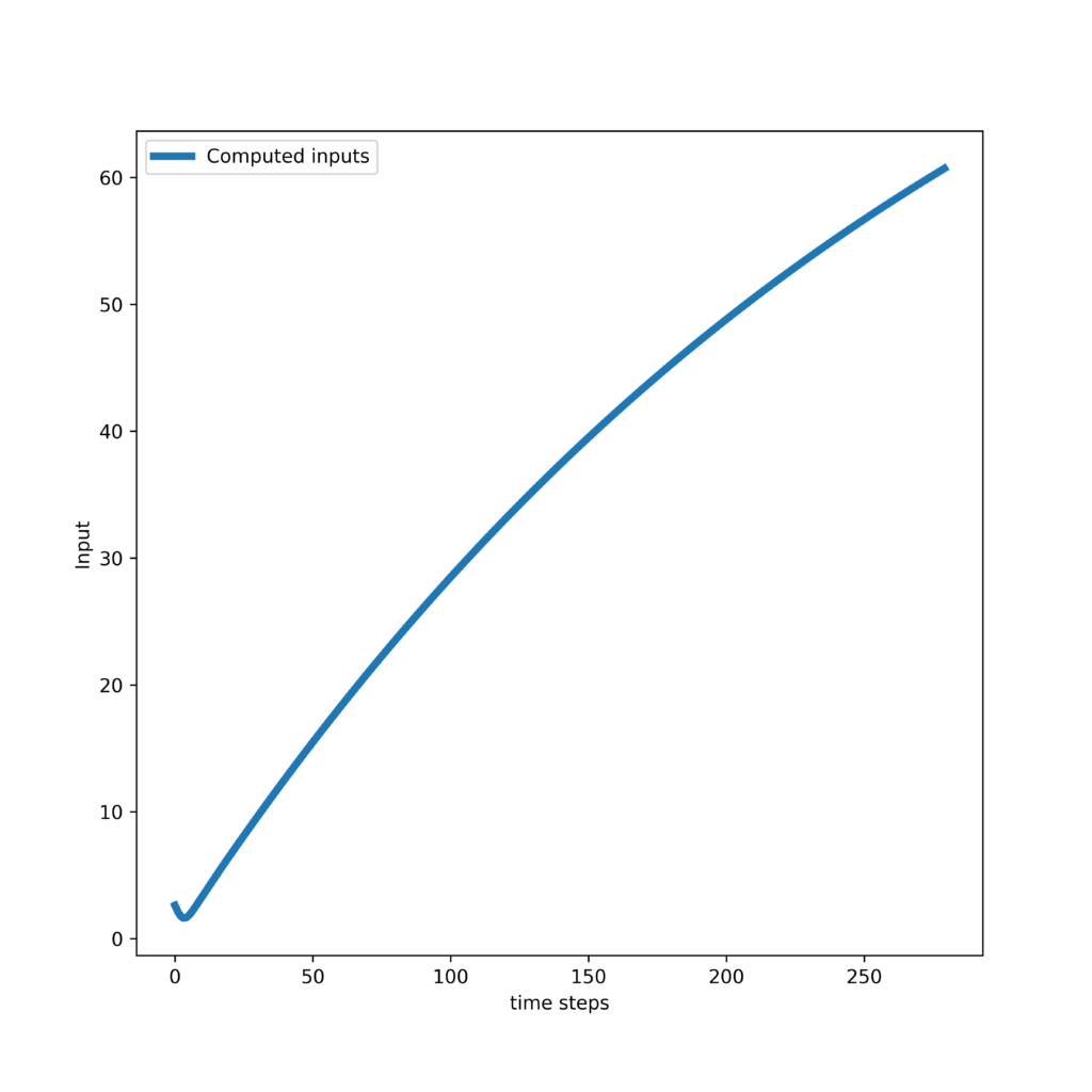
Thirdly, we present the results obtained by tracking an exponential trajectory. The response of the controller and control inputs are shown in the two graphs given below.
Python Implementation of Model Predictive Controller
All the codes presented here are posted on the GitHub page. The following code presents an implementation of a Python class that implements the model predictive controller.
import numpy as np

class ModelPredictiveControl(object):

    # A,B,C - system matrices
    # f -  prediction horizon
    # v  - control horizon
    # W3 - input weight matrix
    # W4 - prediction weight matrix
    # x0 - initial state of the system
    # desiredControlTrajectoryTotal - total desired control trajectory
    #                               later on, we will take segments of this
    #                               desired state trajectory

    def __init__(self,A,B,C,f,v,W3,W4,x0,desiredControlTrajectoryTotal):

        # initialize variables
        self.A=A
        self.B=B
        self.C=C
        self.f=f
        self.v=v
        self.W3=W3
        self.W4=W4
        self.desiredControlTrajectoryTotal=desiredControlTrajectoryTotal

        # dimensions of the matrices

        self.n=A.shape[0]
        self.r=C.shape[0]
        self.m=B.shape[1]


        # this variable is used to track the current time step k of the controller
        # after every calculation of the control inpu, this variables is incremented for +1
        self.currentTimeStep=0

        # we store the state vectors of the controlled state trajectory
        self.states=[]
        self.states.append(x0)

        # we store the computed inputs
        self.inputs=[]

        # we store the output vectors of the controlled state trajectory
        self.outputs=[]
        self.outputs.append(np.matmul(C,x0))

        # form the lifted system matrices and vectors
        # the gain matrix is used to compute the solution
        # here we pre-compute it to save computational time
        self.O, self.M, self.gainMatrix = self.formLiftedMatrices()


    # this function forms the lifted matrices O and M, as well as the
    # the gain matrix of the control algorithm
    # and returns them
    def formLiftedMatrices(self):
        f=self.f
        v=self.v
        r=self.r
        n=self.n
        m=self.m
        A=self.A
        B=self.B
        C=self.C

        # lifted matrix O
        O=np.zeros(shape=(f*r,n))

        for i in range(f):
            if (i == 0):
                powA=A;
            else:
                powA=np.matmul(powA,A)
            O[i*r:(i+1)*r,:]=np.matmul(C,powA)

        # lifted matrix M
        M=np.zeros(shape=(f*r,v*m))

        for i in range(f):
            # until the control horizon
            if (i<v):
                for j in range(i+1):
                    if (j == 0):
                        powA=np.eye(n,n);
                    else:
                        powA=np.matmul(powA,A)
                    M[i*r:(i+1)*r,(i-j)*m:(i-j+1)*m]=np.matmul(C,np.matmul(powA,B))

            # from control horizon until the prediction horizon
            else:
                for j in range(v):
                    # here we form the last entry
                    if j==0:
                        sumLast=np.zeros(shape=(n,n))
                        for s in range(i-v+2):
                            if (s == 0):
                                powA=np.eye(n,n);
                            else:
                                powA=np.matmul(powA,A)
                            sumLast=sumLast+powA
                        M[i*r:(i+1)*r,(v-1)*m:(v)*m]=np.matmul(C,np.matmul(sumLast,B))
                    else:
                        powA=np.matmul(powA,A)
                        M[i*r:(i+1)*r,(v-1-j)*m:(v-j)*m]=np.matmul(C,np.matmul(powA,B))


        tmp1=np.matmul(M.T,np.matmul(self.W4,M))
        tmp2=np.linalg.inv(tmp1+self.W3)
        gainMatrix=np.matmul(tmp2,np.matmul(M.T,self.W4))


        return O,M,gainMatrix

    # this function propagates the dynamics
    # x_{k+1}=Ax_{k}+Bu_{k}

    def propagateDynamics(self,controlInput,state):

        xkp1=np.zeros(shape=(self.n,1))
        yk=np.zeros(shape=(self.r,1))
        xkp1=np.matmul(self.A,state)+np.matmul(self.B,controlInput)
        yk=np.matmul(self.C,state)

        return xkp1,yk

    # this function computes the control inputs, applies them to the system
    # by calling the propagateDynamics() function and appends the lists
    # that store the inputs, outputs, states
    def computeControlInputs(self):

        # extract the segment of the desired control trajectory
        desiredControlTrajectory=self.desiredControlTrajectoryTotal[self.currentTimeStep:self.currentTimeStep+self.f,:]

        # compute the vector s
        vectorS=desiredControlTrajectory-np.matmul(self.O,self.states[self.currentTimeStep])

        # compute the control sequence
        inputSequenceComputed=np.matmul(self.gainMatrix,vectorS)
        inputApplied=np.zeros(shape=(1,1))
        inputApplied[0,0]=inputSequenceComputed[0,0]

        # compute the next state and output
        state_kp1,output_k=self.propagateDynamics(inputApplied,self.states[self.currentTimeStep])

        # append the lists
        self.states.append(state_kp1)
        self.outputs.append(output_k)
        self.inputs.append(inputApplied)
        # increment the time step
        self.currentTimeStep=self.currentTimeStep+1
The definition is straightforward and easy to understand. This class should be saved in the file called “ModelPredictiveControl.py”. Next, we need a helper function for simulating the system response. This function is given below.
###############################################################################
# This function simulates an open loop state-space model:
# x_{k+1} = A x_{k} + B u_{k}
# y_{k}   = C x_{k}
# starting from an initial condition x_{0}

# Input parameters:
# A,B,C - system matrices
# U - the input matrix, its dimensions are \in \mathbb{R}^{m \times simSteps},  where m is the input vector dimension
# Output parameters:
# Y - simulated output - dimensions \in \mathbb{R}^{r \times simSteps}, where r is the output vector dimension
# X - simulated state - dimensions  \in \mathbb{R}^{n \times simSteps}, where n is the state vector dimension

def systemSimulate(A,B,C,U,x0):
    import numpy as np
    simTime=U.shape[1]
    n=A.shape[0]
    r=C.shape[0]
    X=np.zeros(shape=(n,simTime+1))
    Y=np.zeros(shape=(r,simTime))
    for i in range(0,simTime):
        if i==0:
            X[:,[i]]=x0
            Y[:,[i]]=np.matmul(C,x0)
            X[:,[i+1]]=np.matmul(A,x0)+np.matmul(B,U[:,[i]])
        else:
            Y[:,[i]]=np.matmul(C,X[:,[i]])
            X[:,[i+1]]=np.matmul(A,X[:,[i]])+np.matmul(B,U[:,[i]])

    return Y,X

###############################################################################
# end of function
###############################################################################
This helper function should be saved in the file “functionMPC.py”. Finally, below we present the driver code for the model predictive controller.
import numpy as np
import matplotlib.pyplot as plt

from functionMPC import systemSimulate
from ModelPredictiveControl import ModelPredictiveControl


###############################################################################
#  Define the MPC algorithm parameters
###############################################################################
# prediction horizon
f= 20
# control horizon
v=20

###############################################################################
# end of MPC parameter definitions
###############################################################################


###############################################################################
# Define the model
###############################################################################

# masses, spring and damper constants
m1=2  ; m2=2   ; k1=100  ; k2=200 ; d1=1  ; d2=5;
# define the continuous-time system matrices
Ac=np.matrix([[0, 1, 0, 0],
              [-(k1+k2)/m1 ,  -(d1+d2)/m1 , k2/m1 , d2/m1 ],
              [0 , 0 ,  0 , 1],
              [k2/m2,  d2/m2, -k2/m2, -d2/m2]])
Bc=np.matrix([[0],[0],[0],[1/m2]])
Cc=np.matrix([[1, 0, 0, 0]])

r=1; m=1 # number of inputs and outputs
n= 4 # state dimension


###############################################################################
# end of model definition
###############################################################################

###############################################################################
# discretize and simulate the system step response
###############################################################################

# discretization constant
sampling=0.05

# model discretization
I=np.identity(Ac.shape[0]) # this is an identity matrix
A=np.linalg.inv(I-sampling*Ac)
B=A*sampling*Bc
C=Cc

# check the eigenvalues
eigen_A=np.linalg.eig(Ac)[0]
eigen_Aid=np.linalg.eig(A)[0]

timeSampleTest=200

# compute the system's step response
inputTest=10*np.ones((1,timeSampleTest))
x0test=np.zeros(shape=(4,1))


# simulate the discrete-time system
Ytest, Xtest=systemSimulate(A,B,C,inputTest,x0test)


plt.figure(figsize=(8,8))
plt.plot(Ytest[0,:],linewidth=4, label='Step response - output')
plt.xlabel('time steps')
plt.ylabel('output')
plt.legend()
plt.savefig('stepResponse.png',dpi=600)
plt.show()

###############################################################################
# end of step response
###############################################################################

###############################################################################
# form the weighting matrices
###############################################################################

# W1 matrix
W1=np.zeros(shape=(v*m,v*m))

for i in range(v):
    if (i==0):
        W1[i*m:(i+1)*m,i*m:(i+1)*m]=np.eye(m,m)
    else:
        W1[i*m:(i+1)*m,i*m:(i+1)*m]=np.eye(m,m)
        W1[i*m:(i+1)*m,(i-1)*m:(i)*m]=-np.eye(m,m)

# W2 matrix
Q0=0.0000000011
Qother=0.0001

W2=np.zeros(shape=(v*m,v*m))

for i in range(v):
    if (i==0):
        W2[i*m:(i+1)*m,i*m:(i+1)*m]=Q0
    else:
        W2[i*m:(i+1)*m,i*m:(i+1)*m]=Qother

# W3 matrix
W3=np.matmul(W1.T,np.matmul(W2,W1))

# W4 matrix
W4=np.zeros(shape=(f*r,f*r))

# in the general case, this constant should be a matrix
predWeight=10

for i in range(f):
    W4[i*r:(i+1)*r,i*r:(i+1)*r]=predWeight
###############################################################################
# end of step response
###############################################################################

###############################################################################
# Define the reference trajectory
###############################################################################

timeSteps=300

# here you need to comment/uncomment the trajectory that you want to use

# exponential trajectory
timeVector=np.linspace(0,100,timeSteps)

desiredTrajectory=np.ones(timeSteps)-np.exp(-0.01*timeVector)
desiredTrajectory=np.reshape(desiredTrajectory,(timeSteps,1))

# pulse trajectory
desiredTrajectory=np.zeros(shape=(timeSteps,1))
desiredTrajectory[0:100,:]=np.ones((100,1))
desiredTrajectory[200:,:]=np.ones((100,1))

# step trajectory
timeSteps=300
desiredTrajectory=0.3*np.ones(shape=(timeSteps,1))

###############################################################################
# end of definition of the reference trajectory
###############################################################################

###############################################################################
# Simulate the MPC algorithm and plot the results
###############################################################################

# set the initial state
x0=x0test

# create the MPC object

mpc=ModelPredictiveControl(A,B,C,f,v,W3,W4,x0,desiredTrajectory)

# simulate the controller

for i in range(timeSteps-f):
    mpc.computeControlInputs()


# extract the state estimates in order to plot the results
desiredTrajectoryList=[]
controlledTrajectoryList=[]
controlInputList=[]
for j in np.arange(timeSteps-f):
    controlledTrajectoryList.append(mpc.outputs[j][0,0])
    desiredTrajectoryList.append(desiredTrajectory[j,0])
    controlInputList.append(mpc.inputs[j][0,0])

# plot the results

plt.figure(figsize=(8,8))
plt.plot(controlledTrajectoryList,linewidth=4, label='Controlled trajectory')
plt.plot(desiredTrajectoryList,'r', linewidth=2, label='Desired trajectory')
plt.xlabel('time steps')
plt.ylabel('Outputs')
plt.legend()
plt.savefig('controlledOutputs.png',dpi=600)
plt.show()


plt.figure(figsize=(8,8))
plt.plot(controlInputList,linewidth=4, label='Computed inputs')
plt.xlabel('time steps')
plt.ylabel('Input')
plt.legend()
plt.savefig('inputs.png',dpi=600)
plt.show()