Clear Graphical and Mathematical Explanation of Yaw, Pitch and Roll Euler Angles – Part 2

This is the second part of the tutorial on Euler angles and rigid kinematics. These tutorials are important for robotics and aerospace engineers. In this tutorial, we provide a clear explanation of Yaw, Pitch, and Roll Euler angles. We focus on the so-called 3-2-1 Yaw, Pitch, and Roll Euler angles. In the first part of this tutorial which can be found here, we focused on the classical Z-Z’-Z” Euler angles. The YouTube tutorial accompanying this post is given below.

Graphical Interpretation and Geometry of Yaw-Pitch-Roll Euler Angles and Rotations

The yaw-pitch-roll Euler angles are animated in the video shown below. Before continuing to read the rest of this tutorial, first, watch the video given below in order to better understand the geometry of yaw-pitch-roll Euler angles.

The yaw-pitch-roll angles and induced rotations are graphically explained in the figure below.

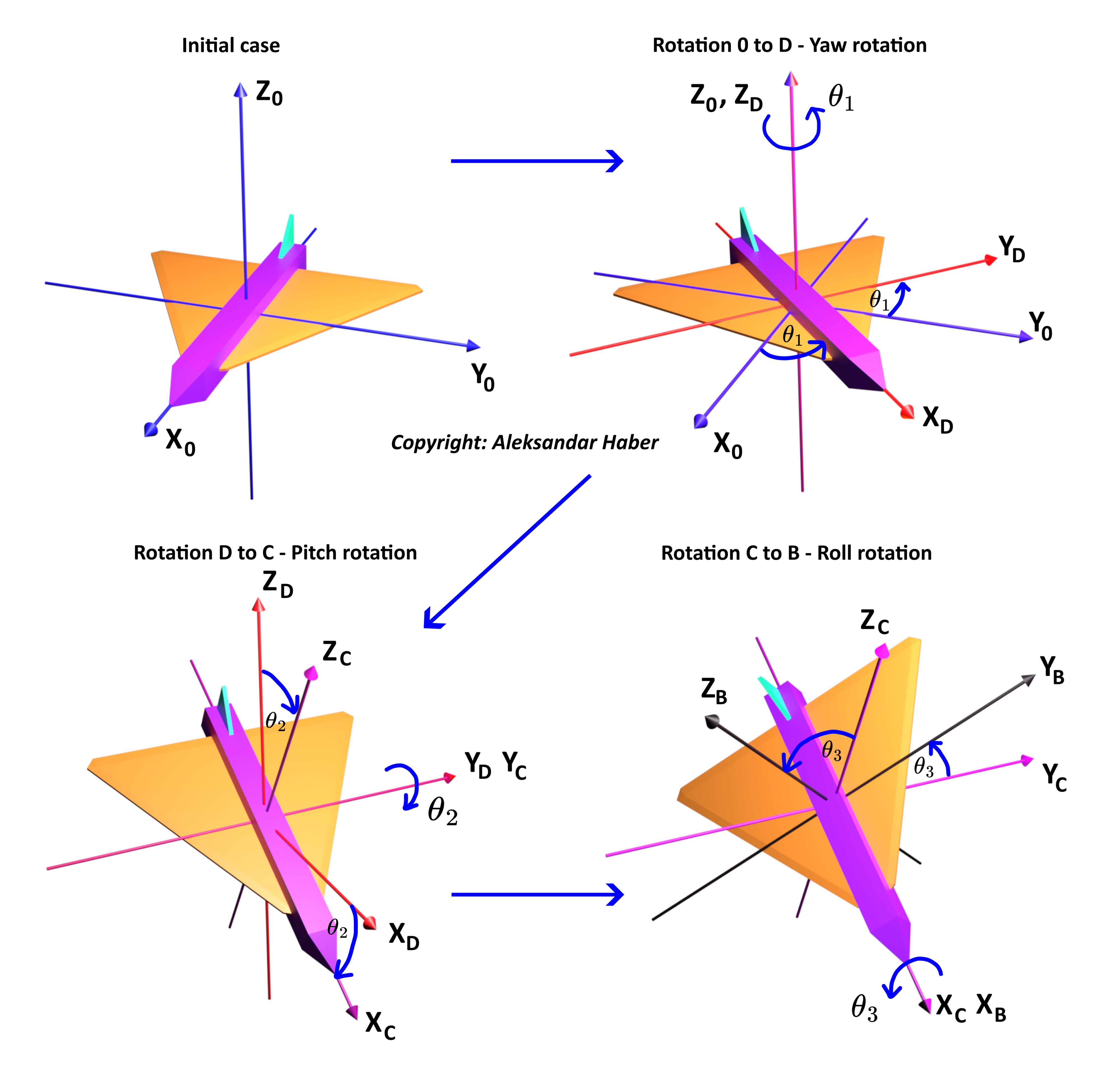
The coordinate system with the coordinate axes is an inertial (fixed) coordinate system.

We have three rotations

1. Rotation around the axis for the angle of . This is the yaw rotation. This rotation defines the coordinate system with the coordinate axes .
2. Rotation around the axis for the angle of . This is the pitch rotation. This rotation defines the coordinate system with the coordinate axes .
3. Rotation around the axis for the angle of . This is the roll rotation. This rotation defines the coordinate system with the coordinate axes .

In robotics and aerospace engineering, coordinate systems are also called frames. The coordinate system is also called the body frame. This is the frame that is rigidly attached to the body of the object and it rotates with the object. The directions of its axes are usually along the lines of symmetry or along the so-called principal axes or principal axes of inertia. We can also interpret the above rotations as follows. The body frame is rigidly attached to the body. After the yaw rotation, the body frame coincides with the frame . After the pitch rotation, the body frame coincides with the coordinate system . Finally, after the roll rotation, the coordinate system is in its final position.

The angles , , and are the yaw-pitch-roll Euler angles. The angle is called the yaw angle. The angle is the pitch angle. The angle is the roll angle.

Next, let us introduce the following notation. Let be a vector. Then, the notation is the notation for the vector expressed in the coordinate system with the following projections in the coordinate system :

(1)  

An equivalent notation is valid for , , and , that is

(2)  

The figure below illustrates the vector in the coordinate system .

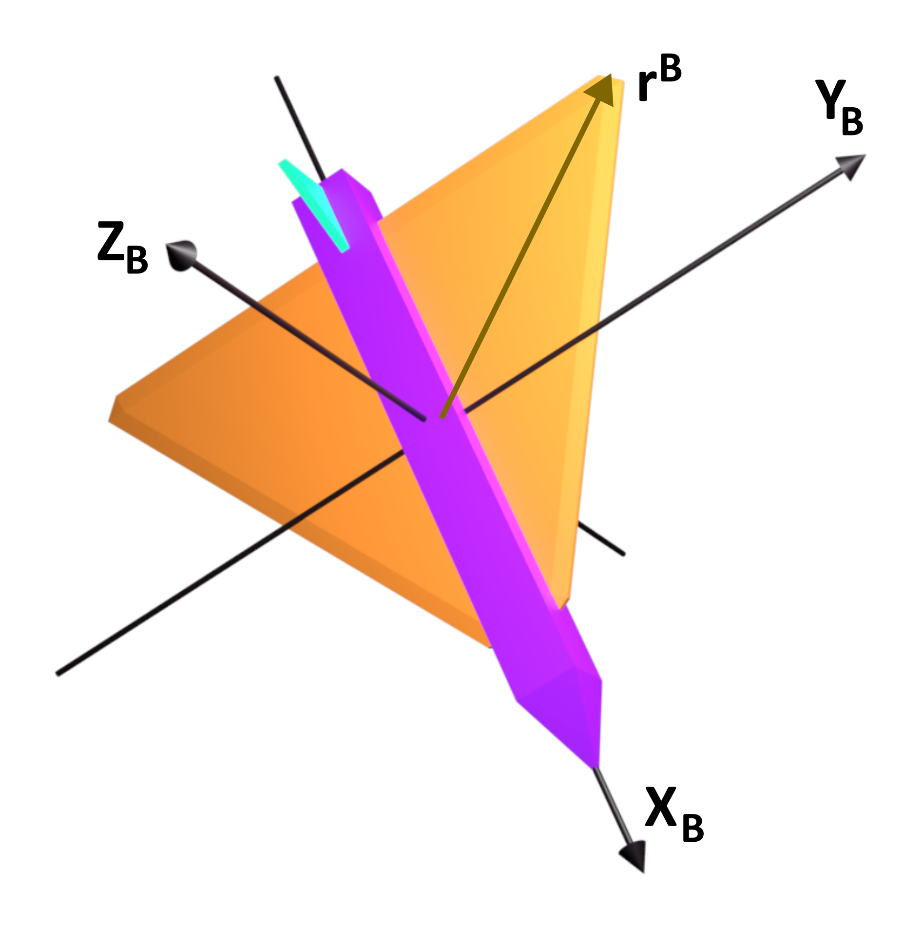
This vector has the following projections in the coordinate system .

(3)  

We consider the following important problem.

We are given the angles of rotation and and we are given the projections of the vector in the coordinate system . That is, we are given . We want to determine the coordinates of the vector in the coordinate system , that is, we want to determine the projections of .

This problem is graphically illustrated in the figure below. We want to find the projections of the vector in the coordinate system .

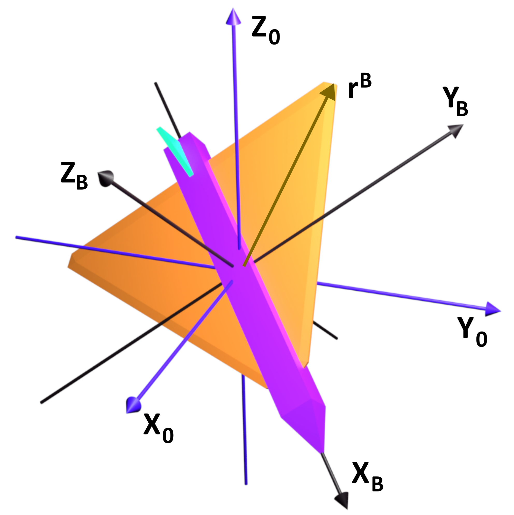
To solve this problem, we need to use rotation matrices that are explained in our previous tutorials, given here, here, and here. Let us now look at the rotation shown in Fig. 1. By using the rotation matrices, we can represent the vector in the coordinate system by using this transformation

(4)  

where is the rotation matrix. The matrix is also denoted by . The notation is the classical notation for the rotation matrix that transforms the coordinate system into the coordinate system . Since the rotation is performed around the axis, according to our previous tutorial on rotation matrices, which can be found here, the rotation matrix has the following form

(5)  

Next, by using the same logic, from Fig. 1. above, we obtain

(6)  

where (or equivalently, ) is the rotation matrix transforming the coordinate system into the coordinate system . Since the rotation is performed with respect to the axis , according to our previous tutorial, which can be found here, the rotation matrix is defined by

(7)  

Finally, by using the same logic, from Fig. 1 above, we have

(8)  

where is the representation of the vector in the coordinate system , and (or equivalently, ) is the rotation matrix transforming the coordinate system into the coordinate system . Since the rotation is performed with respect to the axis , according to our previous tutorial, which can be found here, the rotation matrix is defined by

(9)  

By combining the equations (4), (6), and (8) we obtain

(10)  

The last expression can be written compactly as follows

(11)  

where

(12)  

The matrix is the direction cosine matrix. It transforms the projections of vectors from the coordinate system to projections of vectors in the coordinate system . In our previous tutorial, which can be found here, we explained the main properties of the direction cosine matrix. Next, let us find the explicit form of the matrix :

(13)  

where is the short notation for and is the short notation for .

The equation (11) solves our problem. The Python code given below is used to compute the direction cosine matrix :

from sympy import * 
import numpy as np

init_printing()

theta1=symbols('theta1')
theta2=symbols('theta2')
theta3=symbols('theta3')


Rtheta1=Matrix([[cos(theta1) , -sin(theta1) , 0],
                [sin(theta1) , cos(theta1), 0],
                [0 , 0, 1]
                ])


Rtheta2=Matrix([ [cos(theta2),0, sin(theta2)],
                 [0, 1, 0],
                 [-sin(theta2), 0, cos(theta2)]
                 ])

Rtheta3=Matrix([ [1, 0, 0],
                 [0 ,cos(theta3),-sin(theta3)],
                 [0 ,sin(theta3)  , cos(theta3) ]
                 ])

# double check that inverses are transposes 
simplify(Rtheta1.T*Rtheta1)

simplify(Rtheta2.T*Rtheta2)

simplify(Rtheta3.T*Rtheta3)


# determine the direction cosine matrix
M=Rtheta1*Rtheta2*Rtheta3
# print(M)
# double check the orthogonality
simplify(M.T*M)
simplify(M.T*M -eye(3)) 


# generate the latex script
print_latex(M)