Direction Cosine Matrix Tutorial – Correct Mathematical Explanation -Important for Aerospace and Robotics Engineering

In this tutorial, we introduce the concept of a direction cosine matrix. This matrix is important for mathematically describing rigid body motion, rotations, and other topics that appear in aerospace and robotics engineering.

While preparing a series of tutorials on robotics and UAVs kinematics and dynamics, I realized that in a number of books on robotics and aerospace (from the 80s and 90s) direction cosine matrices and other rigid-body kinematics concepts are explained by using non-standard (from today’s viewpoint) linear algebra notation and conventions. Such conventions were maybe popular during the 80s in the aerospace community, however, from today’s viewpoint they are obsolete. Consequently, even for me, it was challenging to properly decipher how the geometrical concepts from these books are translated into linear algebra and matrix operations. It feels like reading an early math manuscript from the 15th century before standard math conventions were established.

To clarify the main concepts, here is a tutorial I made on direction cosine matrices. Direction cosine matrices are important for robotics and aerospace engineering since they are used to represent a series of rotations around a fixed point. That is, they are used as a tool to represent the orientation of rigid bodies in space. They are a generalization of rotation matrices. Usually, they are expressed as a product of several rotation matrices. In the tutorial, I am using the up-to-date linear algebra standards for transforming geometrical objects into matrices and vectors.

The YouTube tutorial accompanying this webpage is given below.

Direction Cosine Matrix Definition

We consider two coordinate systems and shown in the figure below. The coordinate systems are also called reference frames in aerospace and robotics engineering.

The coordinate system is denoted by the blue color, and the coordinate system is denoted by the red color. The unit vectors that define the axis directions of the coordinate system are

(1)  

On the other hand, the unit vectors that define the axis directions of the coordinate system are

(2)  

Here, we assumed that the coordinate system is rotated with respect to the coordinate system . Also, it is very important to keep in mind that without any superscript or additional notation, the components of unit vectors of both coordinate systems are represented with respect to a third reference coordinate system. For example, if

(3)  

then all 3 projections of and all three projections of are represented with respect to the same coordinate system that is independent of both and . This coordinate system will be denoted by . That is, unless there is a superscript notation, all the vectors are represented with respect to the coordinate system .

Next, consider the figure shown below

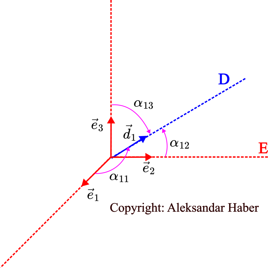
The angles , , and be the angles that the unit vector makes with the unit vectors , , and , respectively. From the figure above, we have

(4)  

Next, let , , and be the angles that the unit vector makes with the unit vectors , , and , respectively. Finally, let , , and be the angles that the unit vector makes with the unit vectors , , and , respectively. We have

(5)  

Now, what is a scalar product of the vectors and ? We have

(6)  

where and are the intensities of the vectors and , respectively, and is the cosine of the angle between the vectors and . Since both and are unit vectors, we have

(7)  

In addition, we have

(8)  

By substituting the last two equations in (6), we obtain

(9)  

Consequently, all the cosine terms in the equations (4) and (5) can be interpreted as the scalar products of and , .

Next, we introduce the direction cosine matrix:

(10)  

The direction cosine matrix can also be expressed as follows

(11)  

where the “dots” are used to denote the scalar product of vectors. Here, it is also important to observe the following. We can also represent the unit vectors , , and , as follows

(12)  

Direction Cosine Matrix, Orthogonality, and Determinant

At the beginning of this tutorial, we explained that all the components of unit vectors of both coordinate systems and should be represented with respect to some third coordinate system independent from the coordinate systems and . The third coordinate system is denoted by . In this coordinate system, the unit vectors have the following components

(13)  

For example , , are the projections of the unit vector onto the axes , , and of the coordinate system . Similarly, , , are the projections of the unit vector onto the axes , , and of the coordinate system . That is, the unit vectors of both coordinate systems are represented in .

Next, let us consider the equations (4) and (5) once more

(14)  

How can we write these equations in the matrix format by using the direction cosine matrix?

By using (13), we can represent the first equation in (14) as follows

(15)  

By using the same idea, we can represent two other equations in (14), as follows

(16)  

The last two equations can be written compactly as follows

(17)  

The last equation can be written compactly in the matrix form

(18)  

where

(19)  

and is the direction cosine matrix defined in (10). The matrices and are formed by placing the corresponding unit vectors next to each other. The meaning of the equation (18) is that we can take the unit vectors corresponding to the coordinate system, and we can transform them into the unit vectors of the coordinate system . Here, we should keep in mind that and are used to denote the matrices composed of unit vectors, and and are used to denote the corresponding coordinate systems.

On the other hand, let us rewrite the equations (12), again

(20)  

From these equations, we can use the identical procedure to the procedure used to derive (18) to derive the following matrix equation

(21)  

Let us next substitute the equation (21) in the equation (18), as the result, we obtain

(22)  

From the last equation, we obtain the following equation

(23)  

This means that

1. The matrix is the orthogonal matrix.
2. The inverse of the matrix is its transpose.

Furthermore, we can show that the determinant of the matrix is equal to . From (23), we have

(24)  

From the last equation, we have

(25)  

From the last equation, we can conclude that the determinant of can either be or . However, it can easily be shown that for the right-hand-sided coordinate system, this determinant should be equal to .

Using the Direction Cosine Matrix to Transform Vector from One Coordinate System to Another

Let us consider an arbitrary vector with the projections in the coordinate system

(26)  

First, let us compute the projections of the vector onto the coordinate system . We want to represent the vector as follows

(27)  

where , , and are the projections of the vector onto the axes of the coordinate system . These projections can easily be computed as follows

(28)  

Now, let us introduce the following notation

(29)  

This notation represents the vector in the coordinate system . By using this notation, we can write the equation (27), as follows

(30)  

On the other hand, we can represent the vector in the coordinate system :

(31)  

where

(32)  

and we can introduce the following notation

(33)  

Similarly to (30), we have

(34)  

Our goal is to find an equation that will transform directly to . Let us start from the equation (30)

(35)  

By substituting from the equation (21) into this equation, we obtain

(36)  

On the other hand, the equation (34) gives us the following relationship

(37)  

From (36) and (37), we have

(38)  

Since the matrix is invertible (non-singular) from the last equation we obtain

(39)  

The last equation is very important. It tells us how to transform the projections of a vector from one coordinate system to another. If we know the projections of the vector in the coordinate system , we can multiply the vector represented in the coordinate system by the direction cosine matrix to compute the representation of this vector in the coordinate system .